Lauren Abrahams

Lauren Abrahams is a student at University of Wisconsin - Madison currently completing her research at Yale University under Dr. Maureen Long.
My research will be analyzing the mid-lithospheric discontinuity (MLD) beneath the central United States. The MLD is a decrease in seismic velocity in the internal lithosphere. Using data from 6 stations I will be able to use receiver functions to analysis the MLD. Currently we are unsure what is causing this change in velocity but some ideas to explain it in the past have been because of the orientation of anisotropic minerals due to strain from past deformation. The lithosphere beneath the United States has been through a large amount of deformation, forming the North American craton, which supports this idea. Doing more research on the MLD will hopefully improve the understanding of the craton formation and modifications.
Ending the Summer right with more Results and Fieldwork :)
July 29th, 2015
Sadly the summer is getting closer to ending. So I’m ending it the best way a geophysicist knows how, doing more fieldwork. Next week I will be helping my mentor Maureen and a few other undergrads show high school teachers how to deploy seismometers. We hope to get the high school teachers excited about geology and hopefully pass the excitement on to their students and community. We will travel around Connecticut and in 4 days we hope to install at least 4 stations. These are Maureen's personal seismometers and she hopes to make a straight array of 15 seismometers across Connecticut.
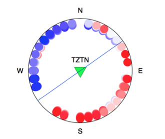
This week I’ve been working on finishing up my project. After creating Receiver Functions I used that data to create Rose Diagrams. In my last blog I talked about how Receiver Functions are sorted by back azimuths, where 0 degrees is on the bottom and 360 is on the top. The Rose diagrams takes a small time section and essentially cuts it out. Then it plots the back azimuths not in a line but in a continuous circle increasing degrees clockwise. In the receiver functions I picked time windows that I thought showed a negative phase in the radial component or a 2 lobed or 4 lobed feature in the transverse component. A 2 lobed feature is a feature that changes from negative to positive or positive to negative velocity after 180 degrees, similarly, a 4 lobed feature does the same only every 90 degrees. A lobed feature indicates that there may be an anisotropic layer.
The goal is if I find a negative phase in the radial component and a lobed feature in the transverse component after the Moho (usually located around 6 seconds) to indicate there might be a MLD. I also modeled much of the crustal structure (before the Moho). There was a lot of possible anisotropy within the crust especially in the stations located on the Appalachian Mountains.
This is station TZTN. I first looked at the radial component and found a large negative phase that was seen through multiple back azimuths. I created a blue box of the time window I wanted to look at and then attempted to place the same time window on the transverse component. It is hard to tell through the Reciever Function diagram where any anisotropy is present.
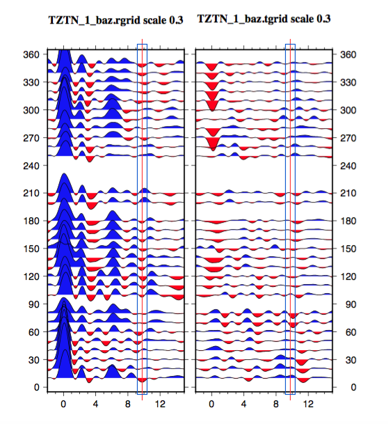
However, when I then created a Rose diagram of the transverse component within that time window you can easily see that there is a distinct difference every 180 degrees. At depth the phases can get less clear because those waves continue to travel up towards the station they interact with higher layers causing some discrepancies.
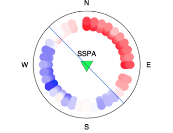
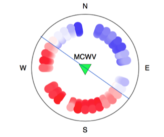
Here are some Rose diagrams I created for the crust structure for stations SSPA and MCWV; you can see that there are very clear differences in lobbed features. These also can indicate anisotropy, however, not MLD because it is not at the correct depths. It is important to analyze the crust to help create models of what the area looks like at depth; the crustal layers could significantly alter how a model will look.
Starting to get Results!
July 14th, 2015
After many weeks of data analysis and preprocessing steps I’ve finally started getting results. I’ve been able to create many different receiver function plots in hopes to find low velocity zones which could be the Mid-Lithospheric Discontinuity (MLD).
The image below is a receiver function I generated. Using 25 years worth of seismograms I sorted the events to help pick out the ones that had visible p-waves and also low amounts of “noise” (excess wiggles on a seismogram not related to the movement caused by the earthquake). None of the seismograms were perfect therefore we stack the seismograms. If there were 5 different events all coming from the same angle they could be stacked. Now those 5 seismograms will not look the same because of the variations with noise. However, when stacked on top of each other and averaged, the noise will cancel out because it is random where the true signal will be amplified.
The image on the left and right are generated from the same seismograms. On the left is the Radial component. The big first blue peak at 0 seconds is the arrival of the P-wave which should mostly only show on the radial component. On the right is the Transverse component, the transverse component measures energy perpendicular to the radial component.
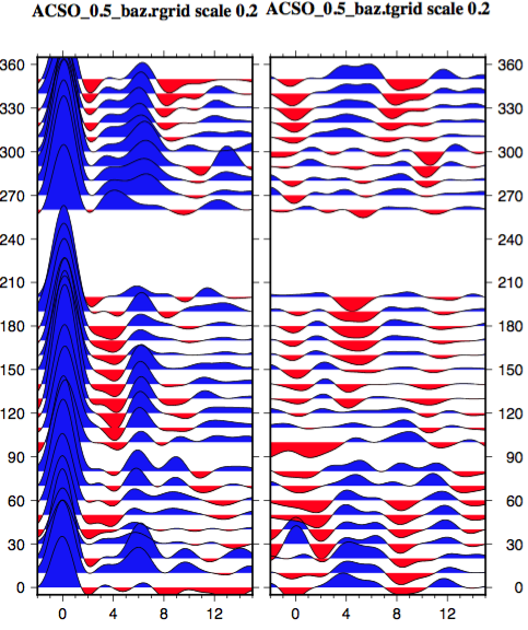
Here on the y axis it shows the back azimuth angle ranging from 0-360. The seismograms with similar back azimuth angles are stacked together because they would have traveled almost the same path to reach the seismometer. On the x-axis is time. The blue shows high velocity and the red shows low velocity. The receiver function is showing how quickly the waves are traveling over time. You can see a blue peak at 0 seconds where the P-wave first arrive. There is another blue peak at around 6 seconds which is the Moho a fast velocity zone. If you rotate the picture seen below, it looks like layers where 0 is the surface of the earth.
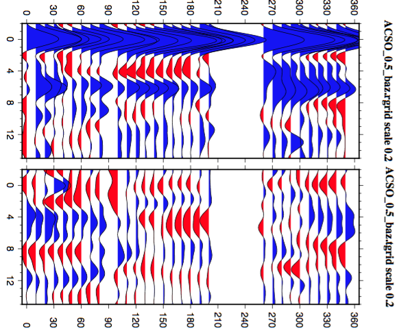
From the surface there are some rock causing red low velocity and then further down from the surface there is the moho causing a blue faster velocity zone.
What I am looking for is a low (red) velocity zone on the transverse component (right hand graph) after we see the Moho. This low velocity zone could be the MLD. Also these images are unmigrated this can cause slight shifts and make the images appear not to have the same velocity zones appear at the same time. We are currently fixing our velocity code to create better models (coming soon :] )
Working in the Field
July 3rd, 2015
I’ve just returned from fieldwork where I was able to travel halfway across the country to deploy and service seismometers. It was hard work digging so many holes and carrying equipment but very well worth it. The MAGIC Array now has 27/28 seismometers deployed and with more seismometers it means more data.
During fieldwork we had to make a lot of stops at different hardware stores. A lot of people were curious as to why we were buying so much cement, sand, fence posts, and other miscellaneous items and started to ask questions. This helped me learn how to communicate our project to the general public. Most people new the basics of what an earthquake was, but not a lot of the key concepts of seismology. The questions I got were: what is a seismometer, does a seismometer create earthquakes, why would we need a seismometer in Ohio.
I would tell people that a seismometer is a machine that can measure earthquakes and vibrations, it does not cause earthquakes but records them when they do occur. Although, Ohio does not get very many earthquakes our sensors are so sensitive that they were able to record the Nepal Earthquake last April. The community seemed excited about our project and that it was going to be in their hometown. I felt that telling more people about our project was almost like outreach; in which it helped educate more people about seismology and get them excited about science.
I really enjoyed being out in the field and learned so many new skills. Below I wrote Lauren’s Guide to Seismometer Deployment a complete list of different things I needed to do while in the field.
Seismometer Deployment
Step 1: Dig a Hole 3ft deep (this has to be deep enough to fit a barrel)
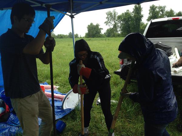
Estimated time: 3-4 hours
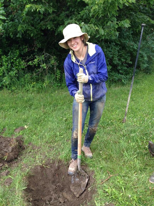
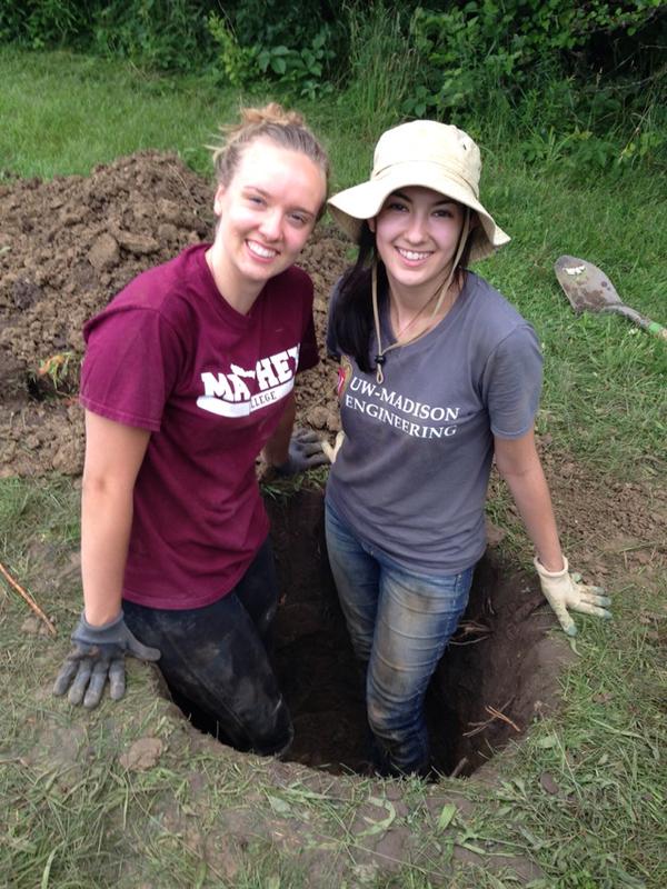
Step 2: Mix and Pour 2 bags of concrete into the hole
Step 3: Place a barrel in the hole add one bag of concrete into barrel
Step 4: Allow concrete to dry, Draw an East west line to orientate the sensor
Step 5: Place seismometer in barrel, orientate and level
Step 6: Dig a shallow hole to house action packer (holds all the electronics)
Step 7: Create trenches that lead from the seismometer to the action packer and a trench leading to where the solar panel will be
Step 8: Create the PVC pipes needed to connect and protect the wires
Step 9: Build the solar panel
Step 10: Place the DAS, Breakout box, Batteries, Power Box, and GPS into Action Packer (follow directions on Station Installation Sheet)
Step 11: Connect wires
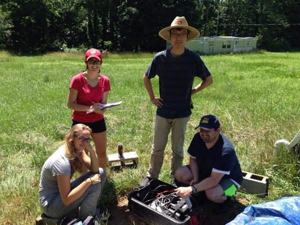
Step 12: Close up barrel to protect seismometer.
Step 13: Bury the seismometer, action packer, and pipes as needed
Step 14: Protect the station by installing a fence if needed
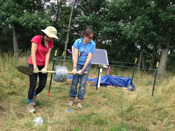
Off to do some Field Work!
June 22nd, 2015
Here’s some clarification on my last post and more about my Project :].
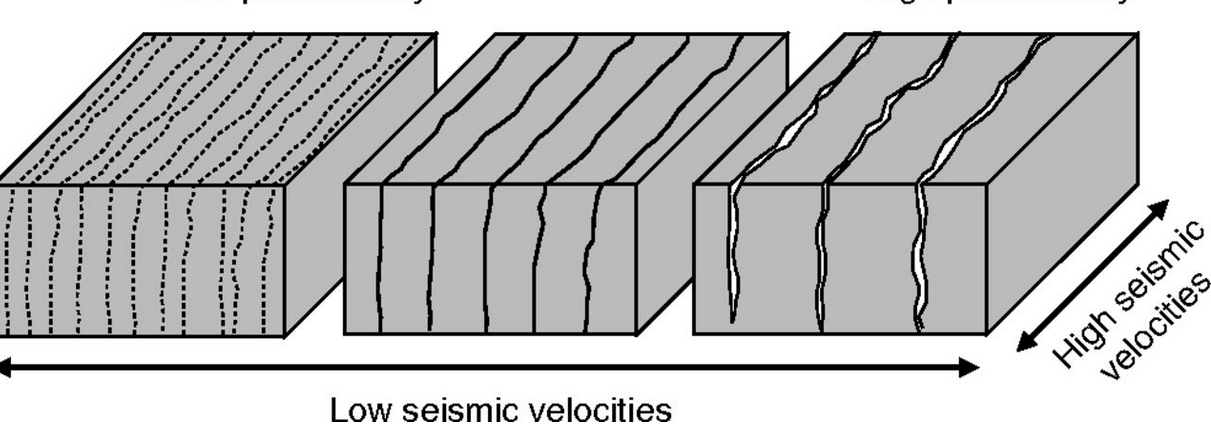
Anisotropy is when the minerals are aligned in one direction. Normally minerals are aligned in random directions (this is isotropic). However, when pressure is applied causing deformation it can cause the minerals to align all in the same direction. Now this causes changes in velocity. If the minerals are randomly aligned the speed at which earthquakes will travel through the material will be pretty uniform in any angle the wave hits. However, once aligned the speed will vary greatly. If the wave is traveling perpendicular, the wave will travel slower. If the wave travels parallel to alignment of the minerals it will travel faster.
Now I’m off to do field work 😊 . I will be helping construct and install 5 seismic stations in West Virginia and Ohio and repairing 7 stations along the way. I’m very excited to start my travels. Below is a map of my journey. I’ll check back in 10 days :]

From Earthscope to field work
June 18th, 2015
The summer sure has been ramping up!
I’ve just returned from the Earthscope conference this past week. Vermont was beautiful and I learned so much. Through the talks and posters I really got a good sense of all the things you can do with seismology. It was a very tiring trip, but a lot of fun to meet other seismologists. My project is Earthscope funded so by attending I was able to learn more about my project and also got to practice talking about what I am doing.
At the beginning of the conference I was pretty worried. I did not know many people there and everyone was much more educated then I was. I pretty much clung to my mentor the first dinner, but slowly started to gain more independence and branch out. This really helped develop my networking skills and gave me more confidence in talking about my research and learning about others. At the end of the conference I felt very confident in the miniature introductory speech I would give to introduce my research.
I am working on the mid-lithospheric discontinuity, which is in the Grenville Front in the grano-rhyolite province. I am examining the MLD because it’s a low velocity zone. This is unusual because the continental lithosphere is very old and stable so there should not be a change in velocity. I am using receiver functions to analyze the area. So far we think this might be due to anisotropy.
It took me 3 days to finally pronounce anisotropy right: ‘an I sought trophy’. I had to repeat this little speech at least 100 times when talking about my research. This makes me excited because if I had read what I just wrote 3 weeks ago, I would have had no idea what any of it meant. I feel like I’ve made so much progress in so little time. I’m extremely exited to start my fieldwork Tuesday and will be traveling halfway across the country installing and repairing seismic stations for 10 days. Wish me luck :]
Nature and Technology
June 9th, 2015
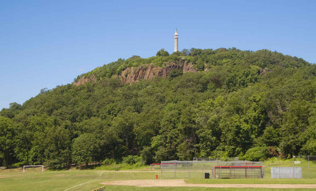
This past week I've had a lot of time to explore Yale campus and the nearby community. On Saturday I was able to hike up East Rock. I definitely underestimated the steepness of the hill. It was nearly a vertical climb 300ft up; however, the view was worth it. It's amazing how quickly the scenery can change from the city to forest here in New Haven.
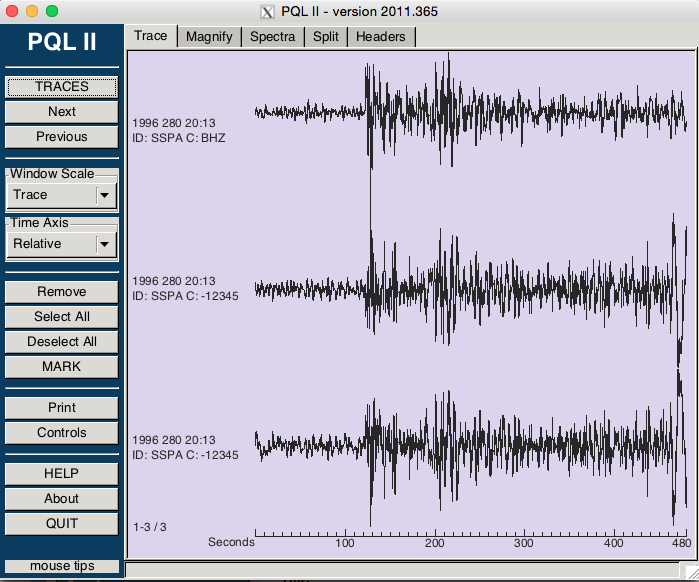
For my reseach this summer I will be working with a variety of programs. So far, I've used 3 diferent programs PQL II, SAC, and SOD. I've started off with raw data that I acquired through the IRIS page and downloaded using SOD. I then used SAC to reorientate the data into radial and transverse components and also to filter the data so the waveforms would be easier to analyze quickly in PQL II. I've spent the majority of my time working with PQL II. It can was frustrating at first constantly crashing on me, however, I found if I load less waveforms (max 5) at once then it won't crash. This makes it take longer to analyze, but once I got into the groove of things I became quicker and quicker. I've been working with a lot of data; some older than I am from 1994! However, I know the more data I look at the better my results will turn out.
Next week I will be heading out to the EarthScope Conference. I am very excited to attend and I know it will be a great opportunity to meet other seismologists.
My First Week at Yale
June 5th, 2015
I've just completed my first week at Yale. It's been so exciting exploring the campus and learning more about my project. I've already looked at thousands of seismograms. I wouldn't be surprised if I started dreaming about them. But, I know all my work will pay off soon when I start creating receiver functions to display my findings.
During this internship I hope to accomplish a lot. A few things I really want to do are learn the terminology seismologists use so I can sound professional, learn networking skills, and also get published. My first 2 goals I've already started working on. Through the papers I have been reading, I’ve learned more and more key terms. As for networking practice, my department has 'tea time' everyday at 3:30 and although I'm just talking to mostly graduate students it has helped me feel more confident and relaxed discussing my research and learning about theirs. Lastly, it will not be easy to get published in the short 12 weeks I am here. Hopefully, I will have enough of a start that I can continue writing up draft papers while I start classes in the fall.
All in all it has been a great start to my internship and I can’t wait to see what will happen next.
Here is a picture of a program I've been using to analyze my data 😊
From Orientation To New Haven
May 31st, 2015
Everyday of orientation was packed to the brim with fun activities. I would never have been able to get this kind of field experience at my home university. Besides the number of hikes we took, I also learned to set up a seismometers and geophones. I've learned so many new things in my first week of the internship I can't wait to see what Yale has in store for me.
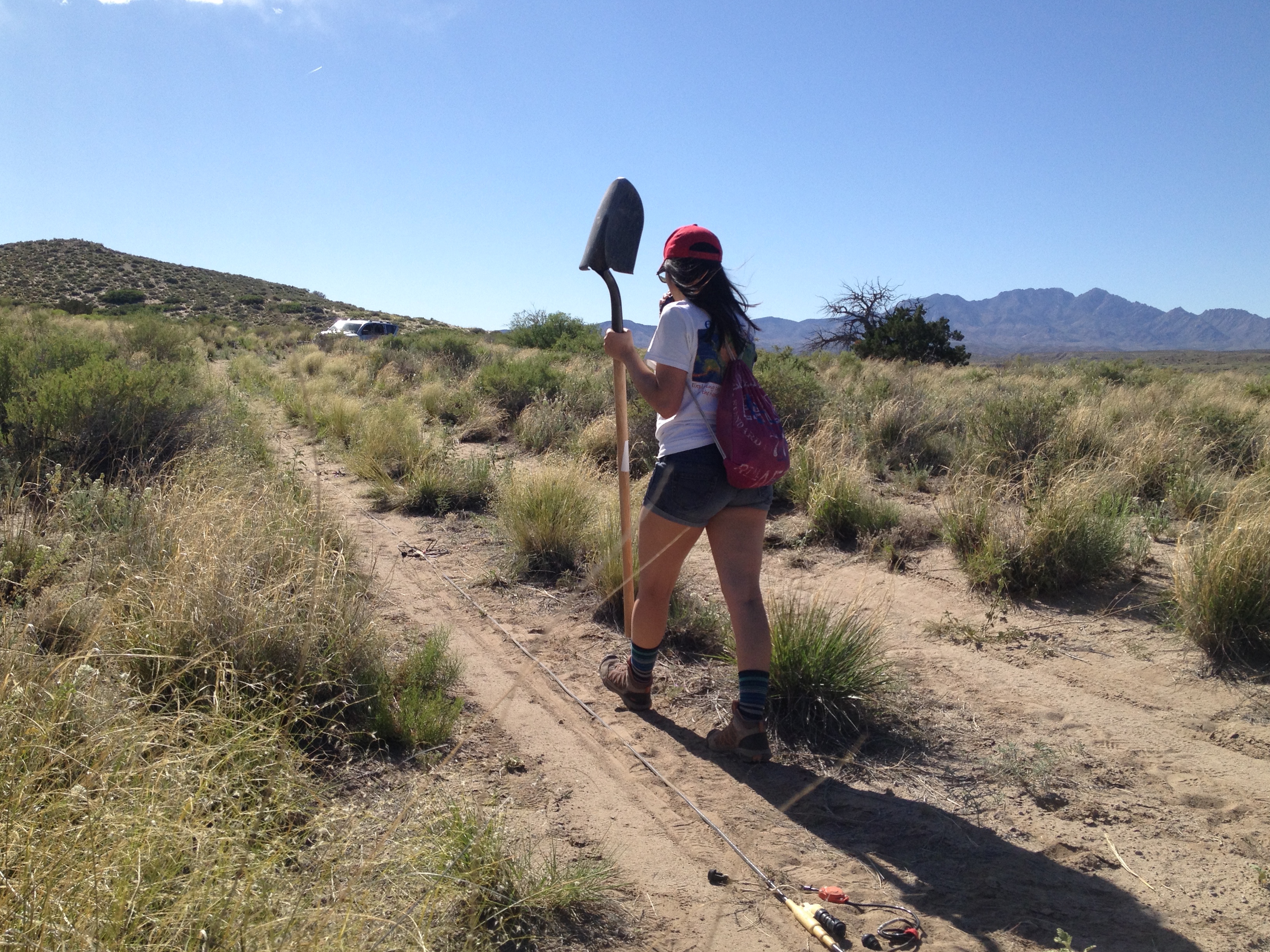
Here's me in New Mexico Checking that each geophone is operational:
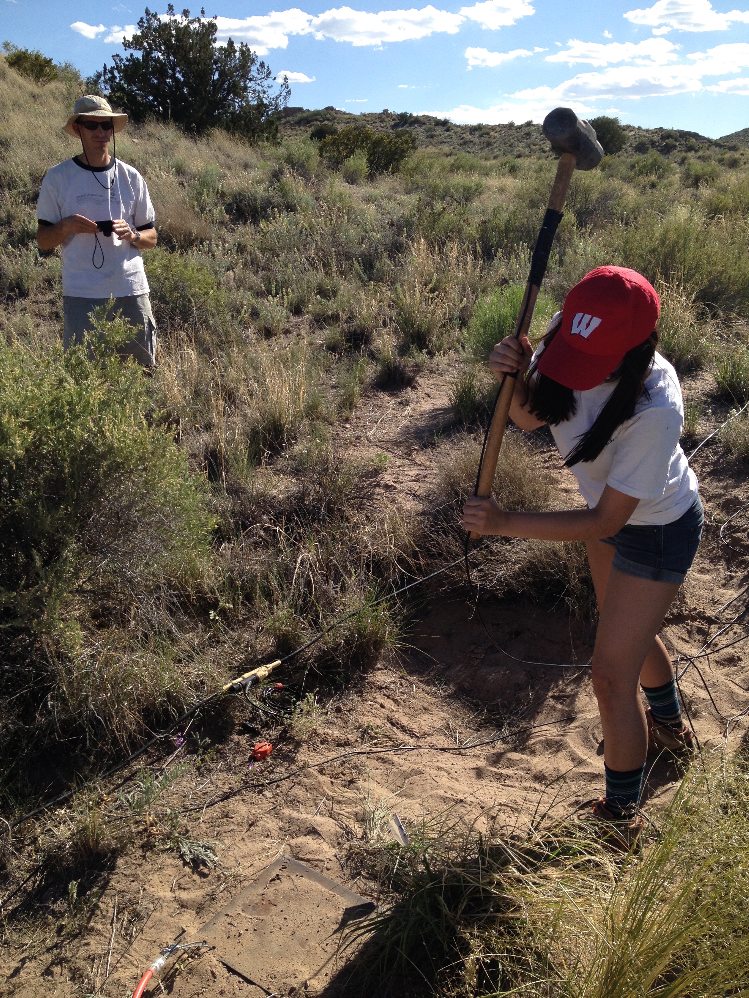
Here's me hiting a metal plate with a sledge hammer to create vibrations in the ground
Orientation Week
May 28th, 2015
Before starting your IRIS internship at your host university, there is an orientation week at New Mexico Tech. During this week, we have a chance to meet other interns, go on hikes, learn geophysics and other computer skills, and have fun with the company of other geologists. Everyone comes from diverse backgrounds and experiences making the orientation more exciting and more meaningful. It has been a great time and I'm not sure the last time I was fed this well. Overall, this has been a once in a lifetime opportunity and I know I will be a better geologist because of it.
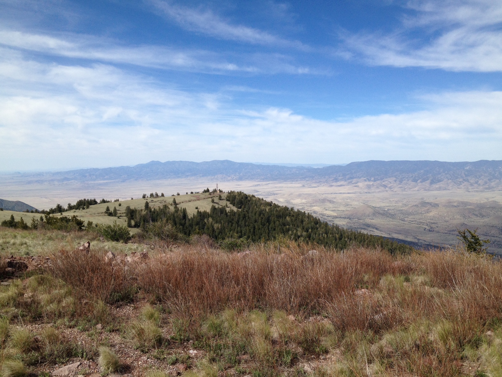
Here's the view at 11,000ft above sea level :]


