Anant Hariharan

December 19th, 2017

**this post is split into two parts for “brevity’s” sake**
 

This was it-the week! 
Unfortunately, but not unforeseeably, my poster only properly came together about 5 days before AGU began, and my talk just squeaked by a day later. I’d been to AGU in San Francisco the previous year, so this really wasn’t my first AGU experience, but it was a more complete and wholesome one. This time, I stayed the whole week, and managed to meet many more scientists both during and outside the conference. 

The IRIS interns were housed in a pretty fantastic hotel about 10 minutes away from the conference, a perfect location if there ever was one. I arrived a day early to get my bearings, head to the convention center to pick up my printed poster (Fabric made for a fantastic albeit expensive material) and upload my slides to AGU’s central database. That night, I headed out to dinner with a few of the interns and got to walk through the streets of New Orleans- it’s hard to describe New Orleans in a way that really does it justice, but the city truly has a distinct personality to it. 

—- Day 1: Monday —-

The first day was intense. 
I went to a few sessions in the morning- a notably excellent one being the first 8:00 am talk from a researcher at Harvard describing her work using triplications to elucidate discontinuities in the transition zone. (Note- taking the derivative of a velocity profile is a really cool, simple way to illustrate the presence of discontinuities with depth!)

I would’ve stopped by some of the posters later, but most of the early afternoon was spent frantically rehearsing my brief 5-minute talk for the Up-Goer Five Session (Describe your research in the ten hundred most common words in English!). Thankfully, the talk -seemed- to go well. I was concerned about the fact that I was bringing a script with me (I didn’t trust myself to not slip up and accidentally spit out the word “tomography”) but it seemed like most of the other speakers had the same idea. 

Being up on the AGU podium was jarring for the first 5 seconds, but seeing my slides on the massive screen was strangely empowering. I eventually got into the swing of things and really enjoyed telling a room full of non-seismologists about my work putting together different models of the Earth’s velocity structure. (of course, not without stumbling on my way back down from the stage).

Later that day, I went to a few other talks (riding the train of euphoria from earlier, I managed to pipe up and pose a decent question at the speaker for one of them, a potential supervisor who I was meeting the next day).

Finally, the night ended with an IRIS reception- it mostly a chance for all us to reconvene for a while (we elected to leave before the formal meeting began) but it was a great event nonetheless.

—- Day 2: Tuesday —-

Tuesday was a blur. 

I capped off the morning by meeting a potential advisor. Naturally, the entirety of our meeting took place in the line for Starbucks’ coffee (she had to run off to a session as soon as she bought some food), but this meant I still managed to get half an hour of an uninterrupted chance to burble on and learn more about anisotropy and the constraints that different things we can get out of a seismic wave impose on it. It’s really only at AGU that you’ll see two people stand in a line for food while pointing excitedly at a piece of paper that one pulls out of his bag, and getting hyped up about what the future holds. It was a good discussion. 

I had several talks today I wanted to go to, but the main event for me was a poster I’d been looking forward to seeing for a long time- one describing a bayesian inversion of multiple seismic datatypes for a full velocity structure! I spent a while here, and it was here that I really realized how varied the reception for posters can be. This one was put together by a professor and truly stood out as perfectly proportioned, formatted, and amazing in every way. As a result, there was almost consistently a flood of people standing by the poster, eagerly trying to ask questions. Someday, I hope I gain the kind of skill to make a poster like that and the reputation attract the kind of audience that the speaker I refer to did.

The night ended with me cautiously going over my speech for tomorrow’s poster session in my head. Stay tuned for more on how that went!

August 20th, 2017

I've ended my project at a highly logical point, and all my codes have been uploaded to GitHub as part of a larger collaborative effort. Onward and over the course of next semester, I'll continue working with my UMD supervisors across a distance to tap even more into the potential of wavelets to elucidate tomographic models, and a paper describing our efforts to do so is now in the works.

It's been a wild ride at UMD (and a week at NMT) over the last 2 months. From digging holes, deploying seismometers, wielding sledgehammers, wading through rivers to profile them, deploying nodes, taking look at fantastic pictures of the deep Earth, and spending weeks basking by the glow of a million open terminals, I'll never forget this summer. While I didn't progress as far on my project as I would've liked, I'm thoroughly excited by what I've managed to learn and accomplish. The Deep Earth has never seemed so tantalisingly accessible, and yet the challenges that prevent us from making unique pictures of it have never seemed so large!

Wavelets are a fascinating tool for signal processing, and I've thus loved the theoretically rigorous aspect of this project. I now greatly appreciate global seismology for it. The perspective I've gained is invaluable, and the advice and tools I've gleaned from my supervisors and team at UMD are facets of a developing researcher's toolkit I can't believe I didn't have.

To all the IRIS interns, grad students, post-docs, and professors I've had the honor of meeting over the last 3 months: It's been an incredible privilege to learn from you, work with you, and do incredible seismology with you. Special appreciation does go to my supervisors at UMD, who've always been available to point me in the right direction and provide me with just the right guidance I need.

And now, I must say goodbye. If you want to learn more about wavelets, I'll be giving a short talk at AGU (ED040) and also presenting a poster (DI012)!

I might add in a special AGU blog post down the line, so stay tuned for that in a few months!

August 5th, 2017

The wavelets have been put in their rightful place at last. We've developed and coded an algorithm that allows a modeller to seek out specific regions of a model by extracting them from the wavelet domain. Since wavelets are geographically localised, we can use them to seek out and compare specific parts of a tomographic model, whether global or regional.

In addition, I've adapted the original algorithm for conducting the wavelet transform on a cubed sphere to improve computational efficiency and more importantly, to run using Python! The key step in doing so involved using MATLAB to generate a wide set of 3-D wavelet basis functions that can be accessed on a sphere.

I've since developed a general set of streamlined functions that work with any input velocity model and allow you to run the wavelet transform on it. Here's an example of what we can achieve if we look at different 'scales' (wavelengths) of a tomographic model.

This is an original velocity model developed by researchers at MIT.

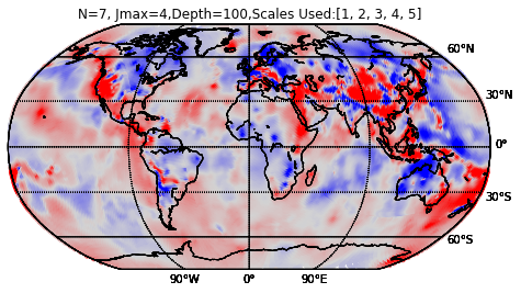
This is the scaling function, or longest-wavelength structure of that model. We can generate this by running the wavelet transform on this model.

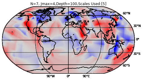
The real power of wavelets for us, however, lies when we combine the same areas of regional and global models. Stay tuned for that- it's only a matter of time.

July 22nd, 2017

As I begin my last month of work, it's time for me to zero in on the true aim of my project. That aim? To develop the first tools to enable the analysis of tomographic models at multiple scales. Let's unpack that a little. 

As I've described in previous posts, tomographic models hold the key to understanding the Earth's interior. In particular, global tomographic models contain a wealth of information about the dynamic processes at work within the Earth's interior. For instance, methods such as spectral analysis and generating radial correlation functions may tell us a) The dominant wavelengths acting within the Earth's interior and b) How similar these wavelengths are at different depths. 

The above results are key in interpreting the data within tomographic models. However, if we wish to conduct the same analysis at regional scales, the way tomographic models are developed prevents truly meaningful comparison. No methods can provide meaningful information on the spectral description of structure within only a certain geographical location- no methods except...

You guessed it- wavelets.  As I've waxed lyrical on them in previous posts, I'll waste no time here. In the past, researchers at Princeton University and other institutions have jointly developed a code to expand Global Tomographic Models into wavelet bases- see my previous post for a figure describing this. It's my job to extend this analysis to focus on retrieving structure within only a certain geographic region. 

This differs quite significantly from my previous training and experience in that it has resulted in work that is far more development-oriented, to my profound delight. I've been forced to eschew the problems of understanding geophysical and geological plausibility and develop the mental acuity to tackle those that revolve around making code easily deployable, computationally efficient, and of course, accurate. This has resulted in a better knowledge of MATLAB and Python than I could ever have hoped; I've been forced to tap into mathematical constructs and software such as sparse matrices, parallel computing and GitHub in order to do a satisfactory job of developing usable code. 

Of course, it goes without saying that this has been accompanied by plenty of head-scratching and late-night fretting. 

Why did the authors index their matrices in this inscrutable manner? Why, oh why, do parallel for-loops not let you interact with variables defined outsode their scope? Why did it crash right -now-? Where did I miss my factor of two within this uncommented mess I wrote 2 days ago? And...will this really work?

I'll leave that fragment of my psyche to rant and rave in the paragraph above. In the meantime, while you're still with me, here's an example of what I'm trying to achieve. I want to recover any desired geographical region of velocity anomalies from the wavelet domain. The first figure on the top-right shows you a 'synthetic', or artifical velocity structure. The middle-right figure shows you a depiction of the structure I -want- to recover from the synthetic structure. Finally, the figure on the bottom-right shows you my attempt to recover it from the wavelet domain, using a mathematical relationship I derived to relate the position of wavelet coefficients to their position in the geographical domain. 

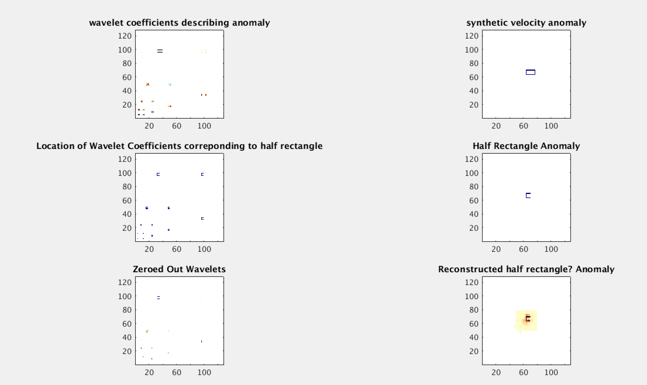
This was a fair attempt; I'm able to recover something resembling half-a-rectangle, but it's still quite poor. Back to the drawing board with you!

(For those of you curious, the issue with this attempt was that I didn't take into account leakage of wavelet coefficients into their 'edges', or the surrounding coefficients. The moral of this story was that empirical relationships can only take you so far- sometimes discretization and computational processing is a limiting factor!) 

And so as I pound away at this keyboard, hoping that the script I've been running for the last 5 hours spits out something worthwhile, I can only leave you with this fond hope: Keep plugging away, and good things will happen. 

Have fun, everyone!

July 9th, 2017

This is the second of a two-part post: the first part explores the necessity for a new way to probe signals within the context of a generalized Fourier Transform. The second part, which is more rooted in examples, explores the difficulty of doing so in a full, spherical Earth and highlights some of the measures that those who map the deep Earth take to remedy it.     

——

    By now, your interest in the wavelet transform is hopefully piqued enough for us to discuss the process of actually applying it to the real Earth. However, this requires us to focus on a new problem- that of the original parametrization in the spatial domain.

     In order to apply the wavelet transform (or any transform, for that matter) we must have the signals parameterized over a coordinate system. The signals that describe the Earth inherently exist in a three or four-dimensional system, and are thus only accurately defined when considered over a framework that is accurate over the surface of the sphere (or more accurately, the ellipsoid).

    A range of attempts have been made to do this. For completeness, I must mention the three most popular bases over which signals that geophysicists deal with on the surface of the Earth are defined: cubic splines, spherical harmonics, and spatially-variant and -invariant grids. Cubic splines simply use represent any single signal as the summation of multiple cubic polynomials constrained at certain boundary points. Spherical harmonics are a similar set of polynomials, Legendre Polynomials, that solve Laplace’s Equation for a range of orders for a given degree; these are just indices used to categorize the different solution. The Spherical Harmonic basis is much more like the fourier domain in that it is orthogonal, and also inherits some of the fourier domain’s convolution/deconvolution properties.

    Intuitively, however, we best visualize functions when considering them as defined over a grid of some sort- this is why latitude and longitude are so popular; they combine a spherical co-ordinate system with the intuitiveness of a grid. Over regional and local spatial scales, this is a perfect solution. However, on a global scale, their inhomogeneity is brought to light, and their coverage is rendered inaccurate, particularly at the poles. As a result, we have to formulate the wavelet transform within what’s known as the cubed sphere- a sphere gridded via a spherical coordinates on 6 separate chunks. This has the advantage of incredibly homogenous coverage, though functions are forced to not be smooth across the edges of the chunks. The image below (Simons et al., 2011) best describes the parameterization we use.

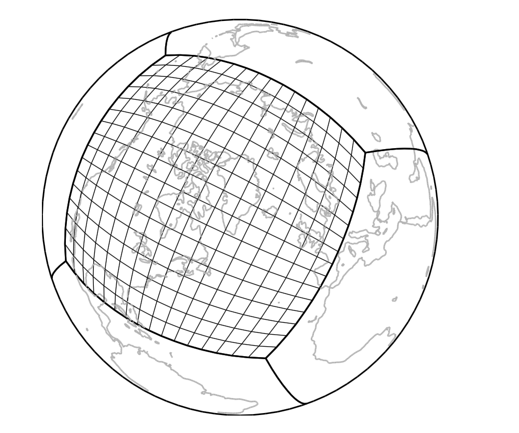
    That’s the hardest part taken care of! Now, we’ve established the parameterization we use to view signals and conduct the wavelet transform in. But how does this help us to understand the Earth? In two ways: Firstly, it helps us understand if natural systems are sparse when viewed in the wavelet basis. And more importantly for our purposes, the localizable property of wavelets in both space and wavelength lets us see how heterogeneous certain functions (such as velocity models) describing the Earth are on certain length scales. This is extremely important! If we can better constrain the dominant length scales of Geodynamic processes acting within the interior of the Earth, we can gain incredible insight onto the physics of the solid Earth and better constrain the source of heterogeneities within the Earth’s interior. For example, the length scale of purely thermal heterogeneities is vastly different from that of thermo-chemical anomalies.

How do we view heterogeneities within the Earth’s interior? With tomography, of course!

Here, I present an analysis of MIT’s 2008 (Li et al.) P-wave tomographic model within the D4 (Daubechies-4) wavelet basis. You can see that the scale-4 processes are more dominant than those at lower scales, indicating that processes on the scale of 20 degrees are more dominant in the lower mantle than those at lower degrees.

This is, of course, only the beginning. Global processes have their appeal, but what about regional scales? What can wavelets tell us when applied to the smaller scales of, say, subduction zones? The journey begins now!

July 3rd, 2017

    This is the first of a two-part post: the first part explores the necessity for a new way to probe signals within the context of a generalized Fourier Transform. The second part, which is more rooted in examples, explores the difficulty of doing so in a full, spherical Earth and highlights some of the measures that those who map the deep Earth take to remedy it.     

———

    As we grow, we inevitably learn that the world is more complex than we think it is. From valence shells to orbitals, from Newtonianism to Quantum Mechanics and from Ray Theory to Finite-Frequency Kernels, the truth gradually unravels as we prove ourselves able to handle it, and we are forced to accept that the natural world is infinitely more involved, chaotic, and exciting than we believed it to be. Consequently, describing it requires us to turn to tools that are equally complex and highlight flaws in their predecessors-exhilaratingly so! Here, I’ll explore the context behind why we need one of these tools: wavelets.

I hope to leave you with a basal excitement for some of the limitations and nuances of the signal processing tools we can employ to describe the Earth.

    Inherent in Geophysical research in the fundamental problem of deconstructing and reconstructing complex signals generated by the Earth. When I began delving into the magical world of signal processing, I rapidly imbibed the ideology that the Fourier transform (a mathematical process that enables us to view signals in both time and frequency domains) was the panacea for any and all problems one might face while trying to analyze a range of waveforms.

    It took me nearly 3 years to convince myself I had even a basic grasp on the Fourier Domain. I believed that this last, magical conceptual leap was finally a solution I could be happy with- a solution that finally elucidated convolution, deconvolution, and a range of operations in both time and frequency domains.

    Oh, how wrong I was.

    While a tremendous breakthrough, the Fourier transform finds itself sorely limited in several regions- the source of this limitation lies within its core ideology: the idea that a basis set of orthogonal sines and cosines of varying frequencies can represent any signal. These sines and cosines are infinitely repeating waveforms- as a result, the Fourier transform is designed to deal with signals that are periodic- signals that repeat themselves after a period of time.

    This means that when signals are impulsive in nature- defined by a sharp burst of energy, or a non-repeating anomaly, the Fourier transform has trouble reconstructing this signal. A primitive manifestation of this issue can be seen in something known as the Gibbs Phenomenon- when signals are forced to rapidly oscillate near sharp discontinuities in the signal.

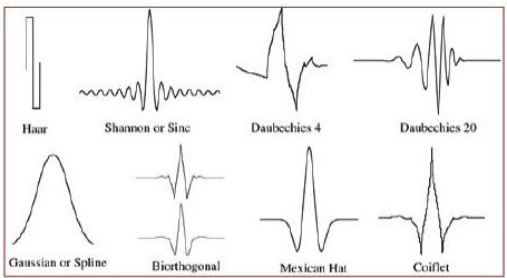
    If we want to deconstruct signals that are localized or vary rapidly in frequency, we’re forced to turn to the wavelet transform- a procedure by which we represent signals using a basis composed of wavelets- pulses which are localized in both time and frequency. These pulses differ in their “scale”, a property loosely related to the duration of the pulse that we might loosely equate to wavelength for a repeating signal, and thus form a basis. Unlike with the rigid sinusoids used in the fourier transform, these basis functions need not necessarily be orthogonal, and can take a range of general shapes, offering greater flexibility.

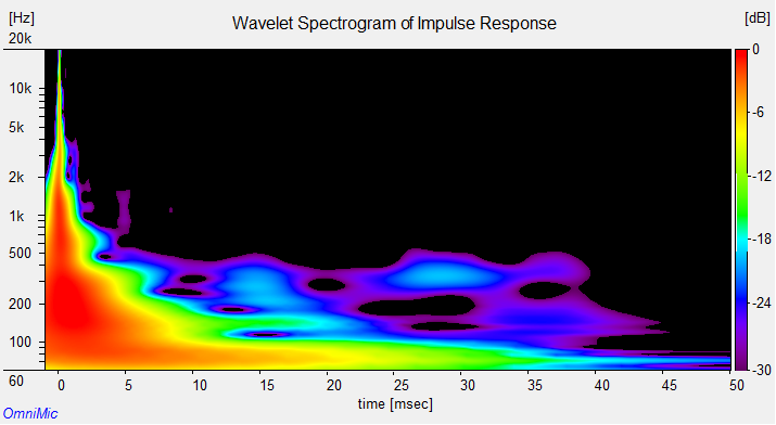
    Although wavelets were used early in the Twentieth Century to analyze quantum systems, their real utility was only explored when engineers realized that wavelets behaved uniquely in the frequency domain, spanning it in a nonlinear fashion. This means that when visualized in Matrix representation, wavelets tend to favor depictions that approach, but don’t quite mimic, sparse matrices. However, if these matrices are truncated, we experience unprecedented gains in computational speed and power. In addition, the wavelet transform can flit more freely between time and frequency domains, favoring neither and allowing joint representations of both, such as in this spectrogram. This process allows us to deal powerfully with signals, such as those from seismic tomography.

    However, the complications have just begun for us. In the field of global tomography, we’re forced to deal with signals that are defined on the surface of the Earth- in other words, defined on a sphere, or more technically, on the ball. This means that the traditional bias functions used to deal with these signals aren’t simply sines and cosines, but Spherical Harmonics, which involve a series of Polynomials known as Legendre Polynomials as basis functions. Here, too, wavelets triumph, as you’ll see next time.

June 10th, 2017

Here’s a brief post focusing on the other, more personal dimension of my time at Maryland, particularly emphasizing how I hope to evolve moving forward. 

It’s been great so far! The Maryland geology building is cozy, and the walls are (naturally) dotted with exhibits of minerals, fossils (and pleasingly), Geodynamic sketches of Earth processes. I began work on Monday, and it’s been a wild ride since, aided by plenty of scripting and esoteric literature.

The latter two mentions lend themselves to my goals for the summer, which follow:

1) To do a solid job.

This goes without saying, but I hope to go above and beyond the call of duty here, taking this chance to probe all corners of this project and get the most I can out of it in terms of knowledge, while being an asset through achieving my mentors’ goal for the summer and helping move their long-term project along its arduous path.

2) To get a better understanding of my research topic, and the general scope of solid-Earth studies.

By the end of the summer, I absolutely need to be able to converse in a scholarly fashion with specialists in global-scale seismology, telling them about what I’ve done and why it’s useful. This is more than a personal goal- it’s absolutely essential for science to evolve.

Towards the latter point, I’m disappointed to admit that several of the data-types used in the tomographic papers I’ve been reading have completely eluded me until now. I’ve been delving into Stein and Wysession to understand concepts such as normal mode splitting. I want to leave this summer as a seismologist perhaps not versed, but at least acquainted with, all the techniques one can use to obtain depictions of the Earth’s Interior, and move beyond the body waves I know and love.

3) To become competent at Python.

I pride myself somewhat on how much I love MATLAB- those light-blue GUI corners, that enigmatic loading screen, those magical arrays… and I want to develop the same love for Python. Being forced to script in it this summer is a great chance to cultivate that love, and it’s high time I began a lasting relationship with the language.

4) To develop a solid time-management scheme.

Perhaps one of the more difficult, yet simultaneously one of the most long-lasting skills to develop. Lists, Calendars or both? Wunderlist or Pomodoro? With all the apps running around, we’re spoiled for choice. I hope to have a scheme set up that enables me to work effectively and efficienty- I’ll need it for Graduate School. 
 

5) Develop the skill of asking Good (and the -right-) questions about papers.

There’s something to be said for people who can delve into a paper and see exactly what makes it tick. I tend to get cowed by the incredible effort that goes into crafting those arguments, and can scarcely move a muscle after reading one. I need to be able to be unafraid of tearing into its innards, finding that crucial assumption that went into the calculations (small angle approximation, anyone?) and boldly asking about it. 

6) Figure out and stick to a good organizational scheme for the waves of literature.

At orientation week, we were exposed to two tools I’m gonna try hard to employ- a cover sheet to use after reading papers, and Zotero, an app for organizing them. The latter might change for me- whether I use Zotero, Mendeley, or Papers, I hope to have papers organized in a pretty database, well-read and easily accessible with the cover sheet stamped on front. Once again, this is a skill absolutely critical to success in grad school, and I -need- to have it figured out. 

June 10th, 2017

Hey, everyone.

This blog entry is going to focus on a general introduction to my research field and briefly touch upon some research developments over the last week.
Expect to see a range of pretty pictures of the Earth’s Interior follow, coupled with intervals of increasingly incoherent seismological rambling. Sound exciting? You’re right- it is!

So, why do we care about Global Tomography at all? What does it even -mean-?

Tomography (etymology: Greek Tomos = section, or slice) roughly describes the act of viewing a 2-D representation of some property of a region, taken along a plane sliced at a specified depth or orientation. 

Within the Earth, the most common types of tomography that we employ are sourced from seismic waves- these waves travel through the Earth’s interior, are affected in some way by the enigmatic material within, and give us valuable information in the form of their attenuation, dispersion, and relative travel times (the time taken for body waves to travel through a material, relative to time they were predicted to travel through the material in). Thus, we have “attenuation” tomography, “surface-wave” tomography, and “travel-time” tomography. There are other kinds, but that scratches the surface well enough. 

For the rest of this post, I’ll refer to travel-time tomography, as applied to image the velocity structure within the Earth. By imaging the P-Wave velocity structure at a range of depths, we can get a window on dynamic earth processes that directly effect P-wave velocity, such as mantle plume upwellings, the presence of anomalously thickening crust, and even the detection of subducted slabs of lithosphere that now sadly rest on the core-mantle boundary- the region known as the “slab graveyard”.

While most seismic deployments typically employ tomography on a “regional” scale, the pinnacle of seismic tomography lies within developing tomography at global scales, where one can compare the entire Earth without bias. However, here lies the problem. At global scales, the problem becomes far more difficult to parametrize, the co-ordinate systems get iffy, the data is far less well distributed (our seismometer coverage within the oceans is -severely- lacking) and our resolution overall grows far weaker. 

However, a range of groups have nonetheless used tomography to generate velocity models of the Earth’s interior. Here's one of the first models ever to do so. (Anderson and Dziewonski, 1984)

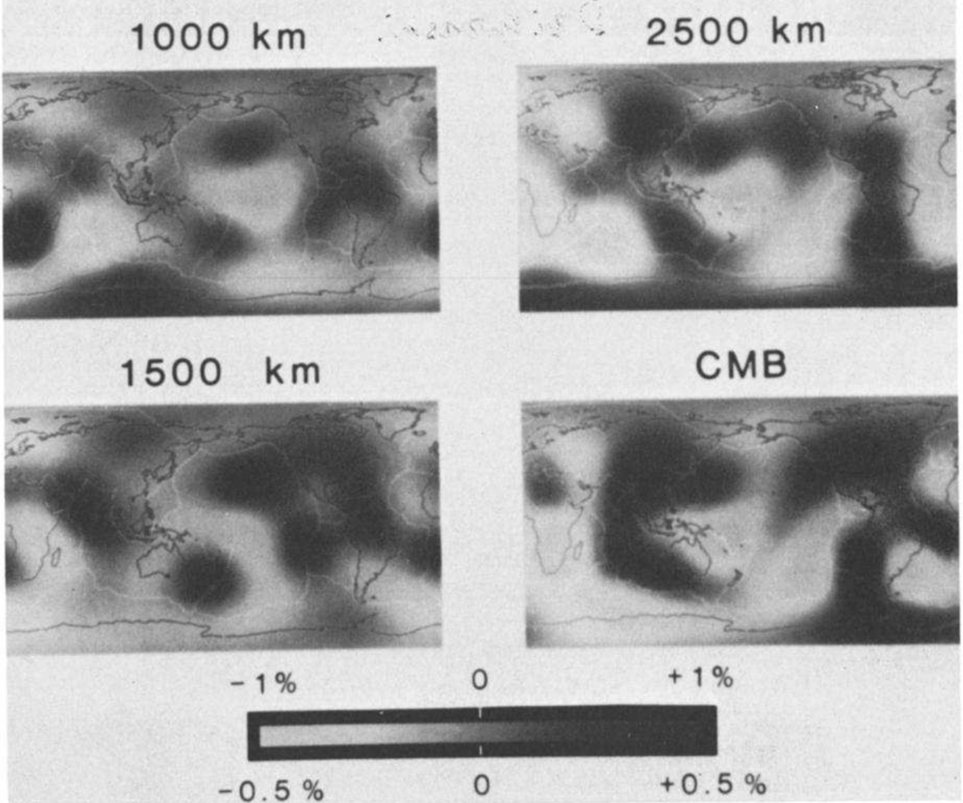
Here's a plot I made of once of the models I'll be analyzing in great depth, made by a group at MIT that only used P-Wave arrival times as their input dataset. We've really come a long way in 30 years, right? Even at a global scale, we can see features such as faults in Tibet using this model. 

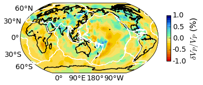
However, all these groups have made models using widely differing methods, and even with widely differing input data! Here’s where I come in. I’m going to be using these models’ velocity structures to explore what they predict, and where they do so. For example, do some models agree strongly on their predictions over a region of overlap despite using different data? Are there regions where different datatypes simply can't be reconciled, and thus should be weighted more weakly in future grand, large-scale inversions?

To better fuel my work, I've been making plots of these models and qualitatively comparing them. I've also been doing some basic analyses on these models- even as they are, their velocity structure can tell us a lot about how they were constructed and where the bulk of their complexity lies. 

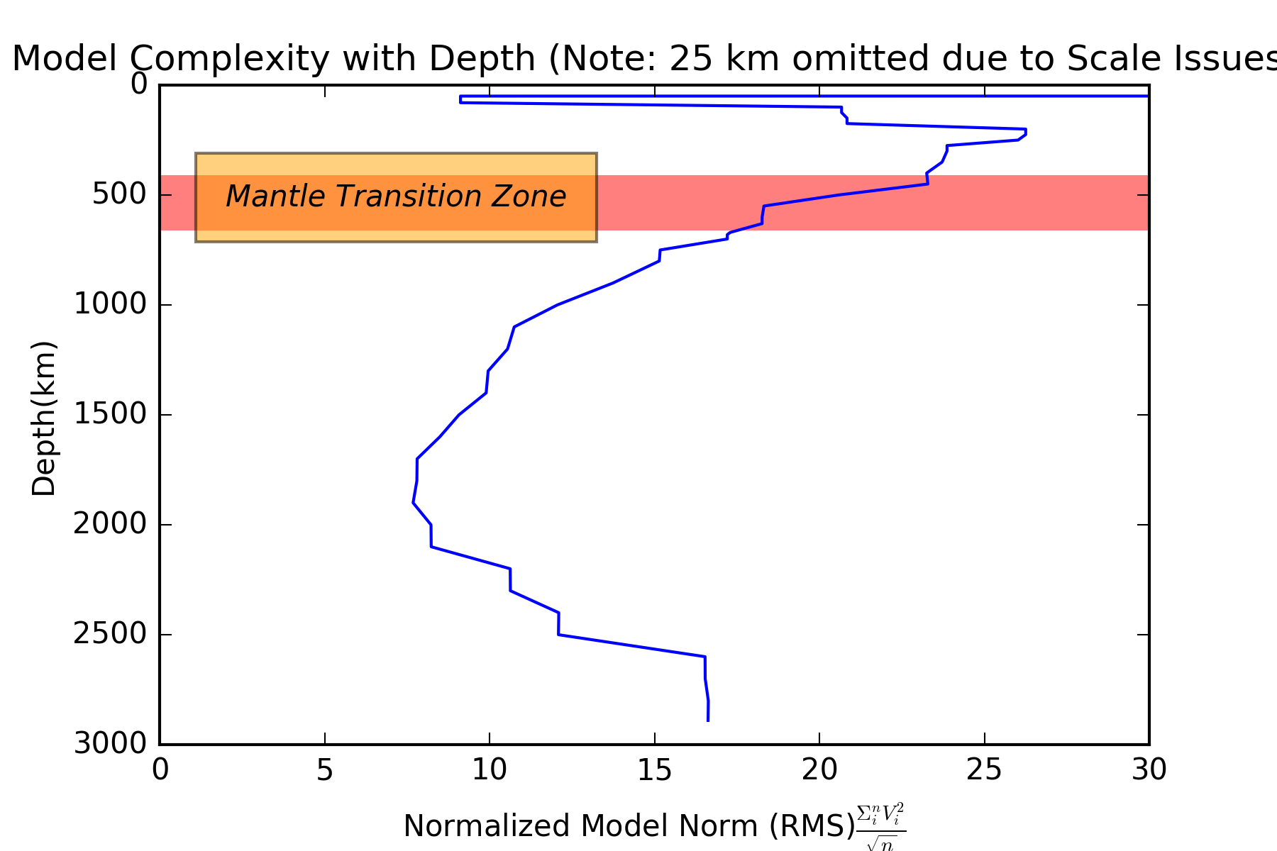
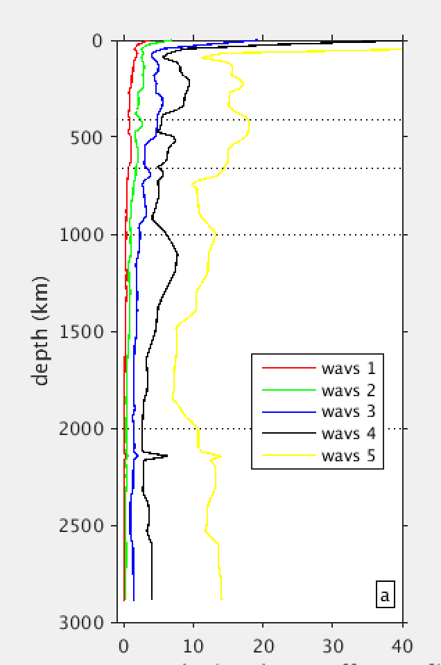
Here's a plot of what is essentially model complexity as a function of depth.
(To calculate this, I simply took the norm of all the full tomographic model's structure at all given depths (basically, the inner product of the velocity anomalies with themselves), normalizing this by the square root of the number of points used)

Even a preliminary analysis shows that key futures about the Earth's interior can be elucidated by looking at the problem from a slightly different angle! As you'll see, earth structure is the most complex (at least, as far as we can probe it) just above the Mantle Transition Zone at 410-660 km depths. Counterintuitively, it also gets more prominent just above the Earth's Core, where studies have uncovered large-scale thermo-chemical heterogeneities! I won't say more for now, but the impact of this deeper heterogeneity is sure to be a focus of mine moving forward. 

That's it for now. If there're any points that I can clarify, comment below and let me now! 

May 31st, 2017

--Testing. Is this thing on?

My name's Anant- I'm a junior and I'll be working on Global Tomography this summer at the University of Maryland.

It's been a great start to the IRIS Internship program. From discussing passive-seismic methods, identifying faults in quebradas along the Rio Grande Rift, and building interactive focal mechanisms, I've never felt more excited about seismology than I do now.

I look forward to using this space to discuss diverse aspects of my research, share preliminary results, and help give you, the reader, a taste of one of the more exciting and timely methods used in global seismology to elucidate the interior of the Earth.