Tara
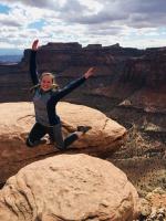
Tara is a student at Brigham Young University currently completing Her research at U.S. Geological Survey - Golden under Dr. Kate Allstadt.
My project will be working on the ShakeMap program developed by the USGS Earthquake Hazards Program. These ShakeMaps provide near-real-time information on significant earthquakes. Currently, this program can provide information on the magnitude, peak ground velocity, peak ground acceleration, and spectral acceleration. I will be working on adding parameters for duration and Arias intensity. These factors can affect the potential for landslide or liquefaction hazards, so this project will be useful in helping us predict these hazards.
Week 10: The Last (full) Week
August 13th, 2018
Week 10
I am reaching the end of my internship, and it is such a bittersweet feeling. I have grown to love all of the people that I have met this summer, and I have really enjoyed my time with the USGS (maybe I'll end up back here one day). At church today, one of my leaders said to me, "I have an inkling that you will be back here permanently." I'll admit, the thought has crossed my mind a few times lately. This place has begun to feel like home, and I think I would really love working with the USGS once I finish grad school. I guess we'll have to wait a few years to find out!
This week, I spent most of my time still trying to read all of the data for the events. I'm telling you, COSMOS is a nightmare to work with. We also ran into problems with Spyder on Wednesday. (Spyder is a Python environment) We had to recreate the main virtual environment I had been using, but when we tried to install Spyder into it, it no longer worked. We could not open any existing projects saved into it or save any new ones. Heather tried to fix it for a couple hours but could never figure out what was wrong. She tried to install Spyder into a new environment on her computer and on another intern's computer, but they were also having the same issues. We're not sure if it's a Spyder thing or if it's just an issue at the USGS. Luckily, I had another environment I was using which already had Spyder installed.
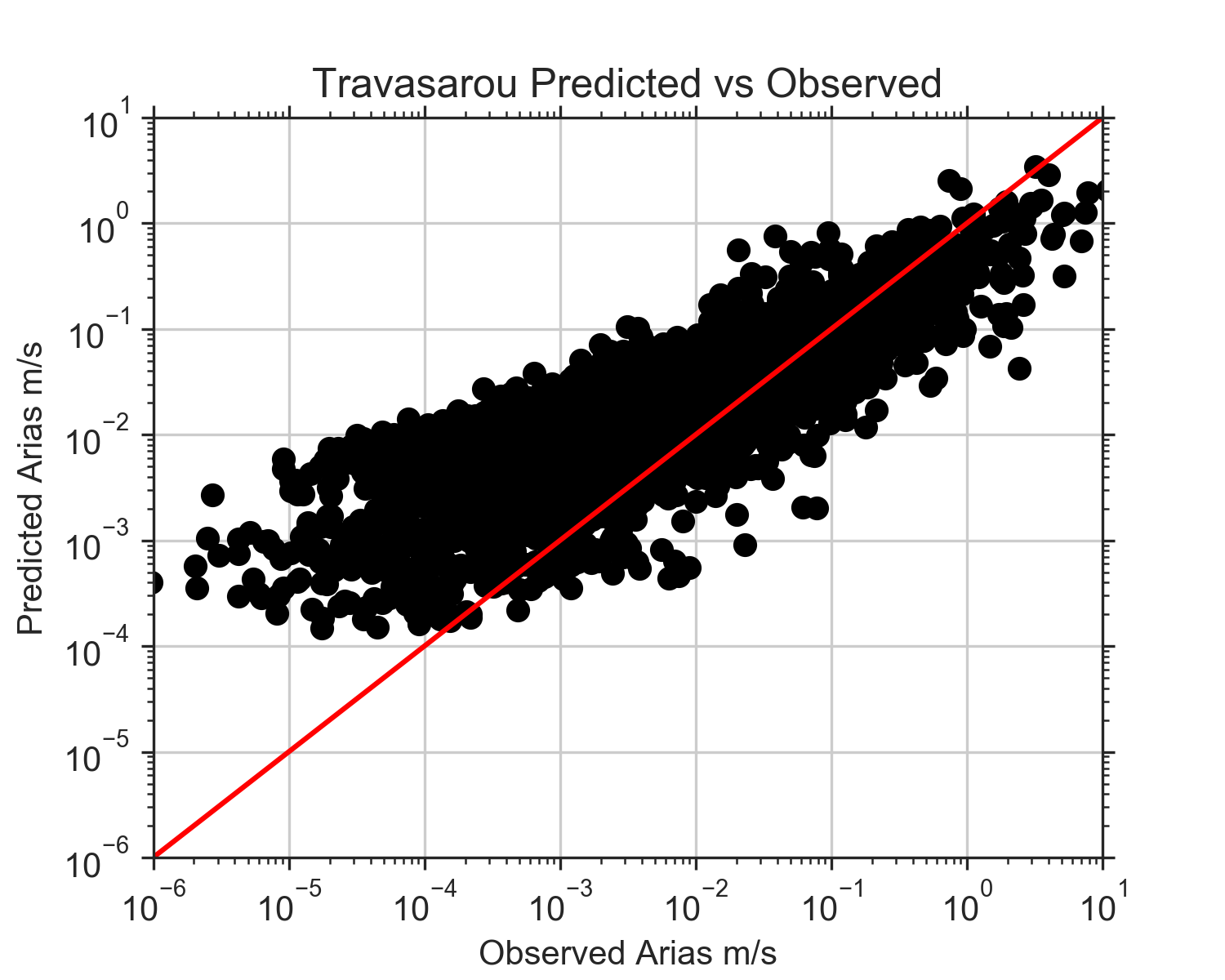
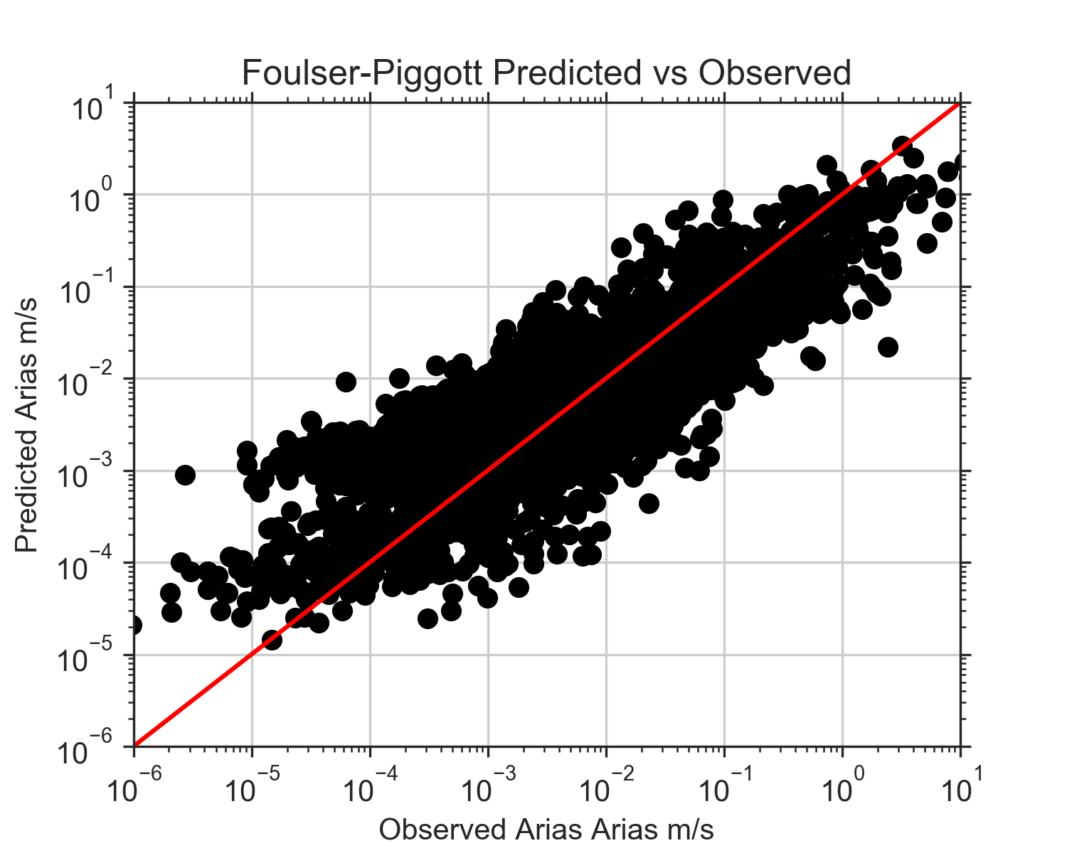
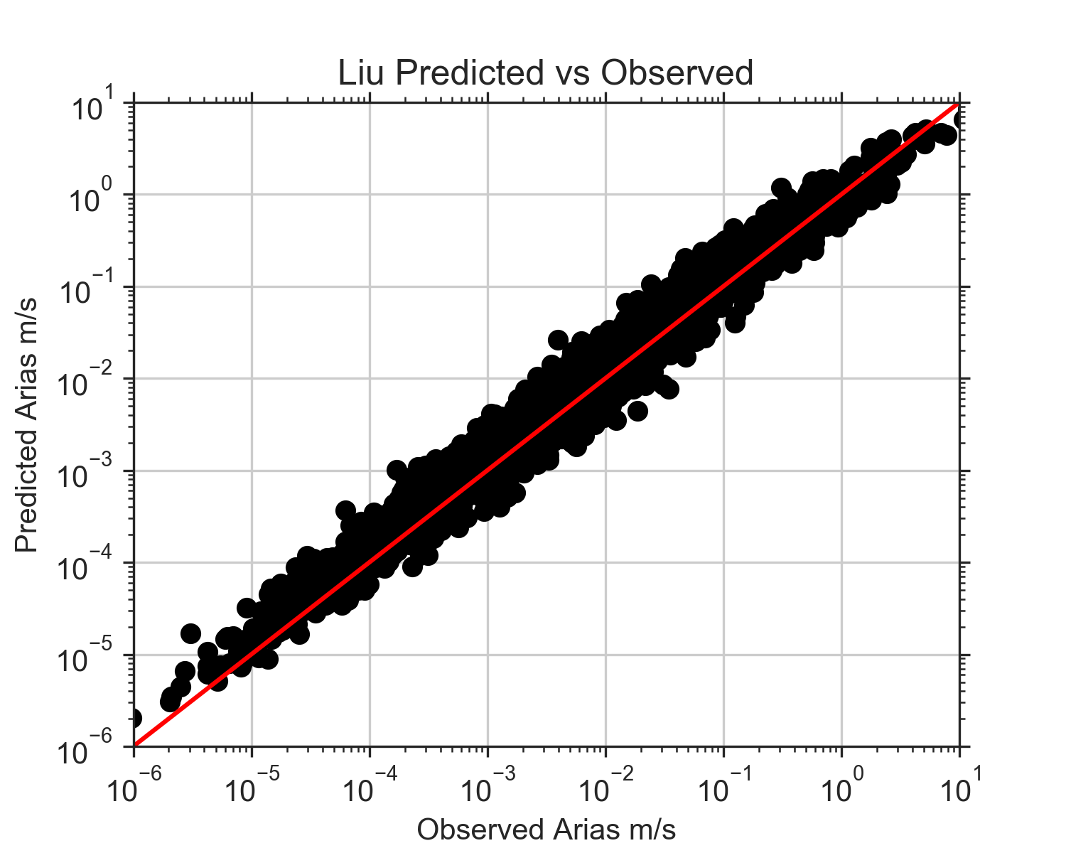
On Wednesday, I also finally got all of the events added except for the Loma Prieta event. I made the judgement call to just scrap that event. We were still having trouble reading it and already had a couple events with similar magnitudes to it. By Thursday, I was able to get all of the rake angles, Vs30 values, and fault rupture distances added to my data frame. Once that was done, I re-ran all the code for the three models and re-made the plots. These next three figures are the observed values of Arias intensity vs the predicted values for each model. The red line in each figure shows where the 1:1 correlation is. If the predicted values exactly matched the observed, they would fall along this line. At lower observed Arias intensities, the Travasarou model overpredicts Arias intensity. Arias intensity is usually lower at greater distances from the fault, so this is consistent with the figures from the previous post where it appeared the model did not work well when considering stations of distances over about 150 km. What's interesting is that it also appears to underpredict slightly at really close distances. The Foulser-Piggott model shows similar trends, except its overpredictions are a little less severe. The Liu model, even after adding a variety of new events, still has a very strong correlation with the observed Arias intensity values. The residuals are much more constrained, and it does not appear to be biased with distance.
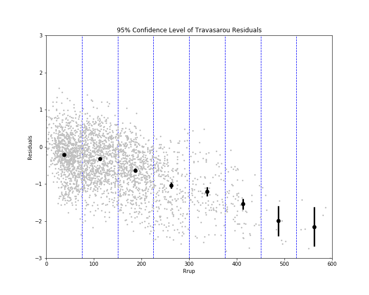
Eric gave me some code to calculate the bias (mean) and inter-event and intra-event residuals (standard deviations) using mixed effects regression. Statistics is pretty abstruse (GRE word) to me, so I don't fully understand what mixed effects regression does. I just know that it gives me a more accurate calculation for the mean and standard deviation. I separated the residuals into bins based off rupture distance ranges or Vs30 ranges. I then plotted the mean for each bin (black dot), as well as the 95% confidence level bars, on the plots of residuals vs rupture distance and Vs30 for each model. 95% confidence means that we are 95% certain that the residuals fall within the given distance (represented by bars) from the mean. If you can't see a bar, that means that it is so small that it is hidden by the mean dot, which indicates the residuals are fairly constrained. To be honest, I'm not entirely sure what the use of these plots will be, but hey, they look cool! I'm sure Eric will explain their significance when he returns to work Monday (he and Kate were gone both Thursday and Friday).

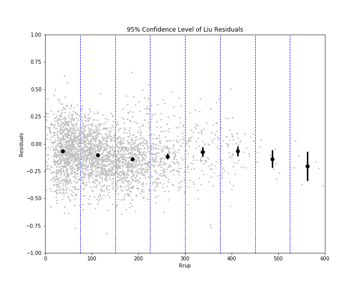
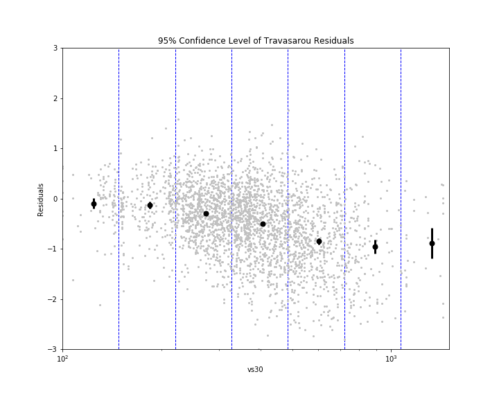
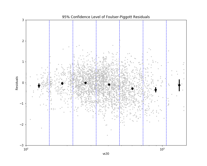
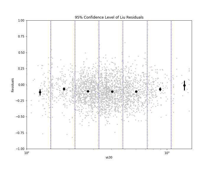
The overall results for the Liu model were quite propitious (GRE word), although a bit shocking. What is surprising about it is that it is not really a ground motion prediction equation (GMPE); it is more of a conversion equation, converting peak ground acceleration (PGA) to Arias intensity. GMPEs have been the main focus of predicting ground motions by many seismologists, but the conversion equation is unequivocally (GRE word) the best method here. You might be wondering, "If PGA and Arias intensity are so strongly correlated, why do we even need to research Arias intensity? Why can't we just continue to use PGA?" That is a fantastic question, one that I myself had! However, we are forgetting that the Liu equation takes into account magnitude and Vs30. Magnitude is not necessarily correlated with PGA. Events of different magnitude could have the same PGA, but the larger one will most likely have a greater duration. Vs30 accounts for the crustal characteristics. If the location is on hard rock, the Vs30 will be higher and the duration lower. However, if the location is on loose soil, the Vs30 will be lower and the duration higher. (This is because waves will reverberate more off loose soil and the duration will be greater) The PGA itself accounts for rupture distance, in a way, because it is affected by distance from the fault. Therefore, PGA and Arias intensity are not directly correlated themselves, but with the help of a few factors, the predictability is unmatched. We have decided to use this model, unsurprisingly I presume, to predict Arias intensity and create ShakeMaps of it.
Next week, I only work through Wednesday, and then I fly back to Utah on Thursday! My focus next week will be on creating a ShakeMap of Arias intensity and on designing my poster for AGU. We might also start incorporating spectral acceleration and spatial correlation, but that depends on how quickly we can get through everything else. My plan is to continue to do some work (voluntarily) for the USGS while I am in Utah, so if something doesn't get accomplished before I leave, I can hopefully work on it during this upcoming semester!
Reflection
This internship has been a beyond incredible experience for me! It is pretty different from the work I have been doing as an undergrad. This project has required a LOT more time (420+ hours), and it has required me to put forth a greater effort into understanding every step of the project. I have been pushed out of my comfort zone in more ways than I can count, such as critically reviewing scientific literature, having my code consistently critiqued, and taking charge of my work without waiting for a step-by-step to-do list from my mentors. (Some of these I am still working on) Every time I finish a task, I have this immediate urge to ask my mentors what to do next, or if I get stuck on an issue, I am quick to ask for guidance. This is my "need for reassurance" quirk coming out, but I think it is also partly due to the fact that, in my meetings with my mentors, our goals were always very limited to what the very next steps were. We hardly focused on the big picture, which made it difficult for me to figure out what next steps I personally could take with the project. However, I am reaching the point in my education/career where I should be expected to start figuring out a lot of this on my own. This is a skill that I have just barely started to grasp, but I know that the experiences I have had with trying to figure it out will greatly benefit me as I head back to school and start preparing for grad school. As a grad student, especially a PhD student (if I choose to go straight into that), my research will be much less guided, and so this is a pretty important skill to start mastering.
Weekend
I spent 3 days baking endless amounts of cookies and writing letters for all of the people I have met during my summer here. They have all touched my life in ways that I never imagined was possible! I am so grateful for the opportunity I have had to spend my summer here in Golden, and thankfully, Provo is only 7 hours away! I'll definitely be returning at some point in the future to visit all of these amazing people. And, who knows, maybe next time I won't be leaving.

Week 9: More events!
August 11th, 2018
Week 9
This week was a little bit slower than last week. On Monday, I continued my attempt at figuring out how to use OpenQuake to run the Travasarou GMPE, but I was running into more errors. I eventually decided to just write the code myself, like I had for the other two equations, using the GMPE in the Travasarou paper. To test that I had coded it up correctly, I recreated figure 2 from the Foulser-Piggott paper. (Foulser-Piggott created this figure using the Travasarou GMPE). My plots looked the same as theirs, so that was nice validation that my Travasarou code was working. I made similar plots for the Travasarou predictions as I did for the Liu and Foulser-Piggott predictions. As expected, the Travasarou GMPE had similar results to the Foulser-Piggott GMPE (the FP GMPE was supposedly just an improvement of the Trav GMPE); however, this model was even worse than the FP model at predicting Arias intensity for stations at greater distances from the fault.
After meeting with my mentors this week, they agreed that something was a little off with the Foulser-Piggot equation (I had some reservations last week with the success of that code). They had me recreate figure 9b from the Foulser-Piggott paper to my equation. My figure did not look quite like theirs did, confirming that there must be a slight error in my code. However, after searching to no avail, I still could not find any discrepancies between my code and the one in the paper. Eric also looked at it for quite a while, but also had no luck. Bruce, one of my other supervisors, discovered that one of my constants was written as v1 instead of V1 (the code has both a v1 and a V1...confusing, right?). This did improve my figure but was still not exactly the same as theirs. Eric attempted to contact Roxanne Foulser-Piggott but has not heard back from her yet. Our assumption is that the figure in her paper must have been made before her code was revised. If she were to make it again using the code in her paper it would probably(hopefully) be the same as ours. The revision I made to my code had very little effect on the figures I made last week with our data, though.
Now that we have the three equations up and working, Eric originally wanted me to start obtaining values for the ROTD50 component of spectral accelerations at different amplitudes. ***Obtaining spectral accelerations will be necessary if we want to add spatial correlation to Arias intensity*** ROTD50 can be a little difficult to comprehend, but I'll do my best to try to explain it. A paper by Boore et al. 2006 stated that "Records of horizontal ground shaking are obtained from orthogonally oriented components, and thus two records are available at each site. There are many ways to use the two horizontal components in ground-motion prediction equations." This is basically saying that at each seismic station, there are two records of horizontal acceleration (and one vertical). These are the three components I have mentioned in some posts over the past few weeks. The two horizontal components are oriented 90 degrees from each other. They could be at 90 and 180 degrees, 45 and 135 degrees, 20 and 110 degrees, etc... These two components can be combined in a variety of ways. A few weeks ago, I calculated arithmetic mean and geometric mean of the components. The two horizontal components can also be rotated throughout a full 360 degrees (while still maintaining their orthogonality). When they are rotated, the acceleration or amplitude values change. The minimum amplitude observed (regardless of which horizontal component it is) while being rotated the 360 degrees would be denoted ROTD00 and the maximum amplitude observed would be denoted ROTD100. Hence, ROTD50 is just the value at the 50th percentile of all the rotated values. ROTD50 is one of the most common intensity measure components used by seismologists right now.
Heather, one of the interns in the office next to mine, has contributed to some code which will compute the ROTD50 for spectral amplitude at any period. However, the code was going to take days to run because it takes quite a while to rotate through all 360 degrees. Eric decided that it would be more useful for us to just work on adding more events to our database than adding spectral accelerations, at least for the time being. The 4 events we have been looking at all range from about a magnitude 6.6 to 6.8. We wanted to get a variety of magnitudes and from different locations to get a better idea of how well the three models work. We decided on adding the Chino Hills(5.4), Parkfield(6.0), Napa(6.0), Loma Prieta (6.9), El Mayor Cucapah(7.2) and Chi Chi(7.7) earthquakes. These are all located in California, except for Chi Chi which is located in Taiwan. I also need to locate a few smaller Japanese events to fill in the lower magnitude range. Downloading the Japanese data was a breeze because all of their data is in the same format and it is very organized. Getting the data for the other events has been a whole other story. I have to download their data from COSMOS, which I have discovered is an absolute nightmare. Their data is already processed when you download it, but the acceleration text files are all in a variety of formats. Even when you think the formats are the same, there are little discrepancies that cause our reader to not be able to read the files. I had to constantly get Heather's help updating our reader so that it could read all of these different files. I still don't have all of them read in yet. I also need to obtain the Vs30 values for all of these new stations and the rupture distances. For the Vs30, I will need to use the global Vs30 map and the coordinates for all of the stations. Hopefully Bruce will get the Vs30 values for me again since my GMT is not compatible with the code. To get the rupture distances, I will need to find fault text files for each of the large events and use our code to calculate the fault distances. For the smaller events, we can just use the hypocentral distance, which is the distance from the station to the initial point of rupture. Next week, I will hopefully be able to finish adding all of the events to my data frame, because I am quickly running out of time to do anything with them!
Reflection
I got my abstract submitted this week! AGU feels so real now, which is kind of terrifying but also really exciting. I feel like I have learned and grown so much over the past 9 weeks. Looking back at my initial goals, I definitely feel like I have been able to accomplish most of them. I've gained SO MUCH experience in programming. I'm pretty much a pro at Python now (not really but compared to week one I am). I've also improved in managing my time and efficiently reading scientific papers. I've read thoroughly over 13 papers this summer and have skimmed a few more. While reading all of these papers, I started to pay more attention to the motivation for the papers. I also started to focus more on the methods and how they can be applied to our work or what their limitations are. This was something I always skimmed over in the past, but now that I am actually applying these papers to my own research, the methods can be pretty crucial to understand. A goal that has developed over the course of my time here has been communicating more effectively, especially with my supervisors. Often times, I will have a question but will have a hard time explaining it to my supervisors. There were mutliple instances where I would ask a question, and then one of them would not understand what I was asking. Then they would try to give the best explanation they could, but I would still be just as confused. This is something I am still working on, but I believe that this has gotten a little better these past few weeks. I've also worked on communicating my project to others outside of work, too. There are a couple people I see weekly who like to ask what I've been up to. At first it was difficult to explain the work I've been doing, but I've been working on coming up with succint explanations. I've also spent a lot of time preparing for grad school. Prepping for the GRE has become a second job. This has been quite arduous (GRE word), but I can see that I have improved a lot! I have also started looking at potential grad schools. The ones I am most interested in right now are the University of Washington, the University of Utah, the Center for Earthquake Research and Information (CERI), and CalTech. I still need to look into the actual professors and what their research focuses on.
Weekend
This weekend, I got randomly sick, so I didn't do too much. I was at work until after 8pm Friday night trying to work with the new data. By the time I got home, I felt pretty worn out, but then I started to feel nauseous and almost passed out. That's why you don't sit a desk for 12 hours, kids! Coincidence? Maybe. Either way, I still felt weak and achy all day Saturday. I still got my weekly dose of ice cream though!
Week 8: Testing GMPEs (Finally)
July 30th, 2018
Week 8
I think this has been one of the most exciting/productive weeks thus far! We are really making progress, which is a huge relief considering I only have 2.5 more weeks here. Is that even real? I've been here so long now that this has become the new normal for me. It's going to be so strange going back to school and leaving all of the new people I have met here...Now is not the time to worry about that though!
This week started out with me finishing up the spreadsheet. (I know, I've been working on this for weeks. It's pretty crucial to the next steps of our project, though.) I still struggled for a bit getting the rest of the Vs30 values from a map. I downloaded the shapefile for the Vs30 map of Japan, but it did not show any Vs30 values when I uploaded it into QGIS. I also tried using Fiona to extract the Vs30 values in Python, but that did not seem to work either. The intern working on Vs30, David, has been using/editing a repository from GitHub which takes shapefiles of geographic locations and converts them to a GMT grid file. I tried using this same code, but it is not compatible with GMT 5 yet (just GMT 4), so it would not work on my computer. One of my supervisors, Bruce, offered to get the values for me on his computer given the coordinates of the stations that needed them. That made my life a lot easier! The last things I had to add to my spreadsheet were fault distances and peak ground acceleration (PGA). Eric helped me write the code for the fault distances, and that was pretty easy. I think we used a GitHub repository called shakemap for that. We just had to input the coordinates of the corners of the faults, which were obtained from a fault text file for each event. The peak ground accelereation is just the maximum acceleration recorded at each station, so that was also a quick task. Once all of that was done, I could start inputing these values into ground motion prediction equations (GMPEs)!
The three GMPEs that we are using are the ones by Liu et al., Travasarou et al., and Foulser-Piggott and Stafford. I started off with the Liu GMPE because it was a fairly simple equation to code up. This particular equation correlates PGA with Arias Intensity, and its inputs are PGA, magnitude, and Vs30. Before using the GMPE on my data, I recreated figure 3 from the paper. This figure plots Arias intensity as a function of PGA for three different magnitudes (4.0, 6.0, and 8.0) and three different Vs30 values (180, 500, and 760). The purpose of this was to insure that my my code was written up correctly. The graphs were basically identical, which was good news!

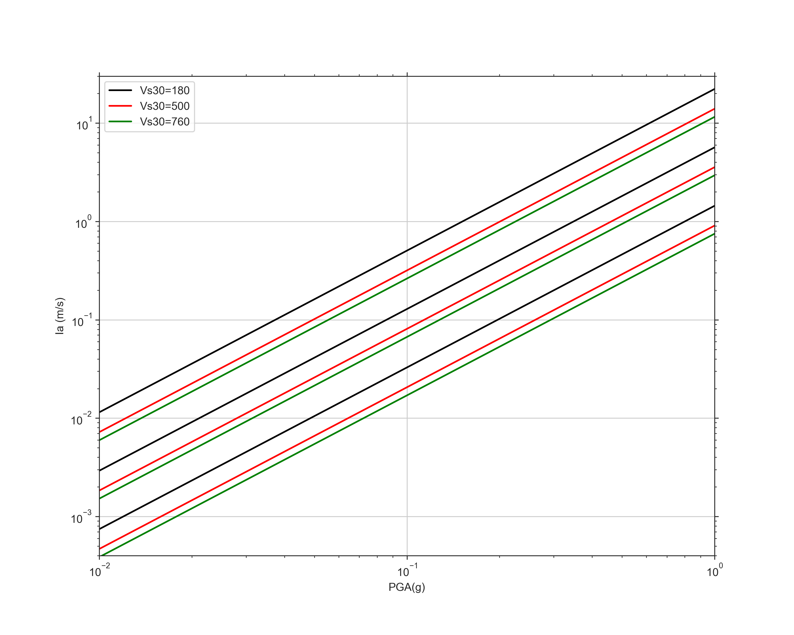
After this verification, I was able to use this on my data. When I first plotted the observed Arias intensity with the predicted values, the graph looked a bit off. The slopes were about the same, but the predicted values appeared about a magnitude greater than the observed ones. It turns out that the Liu GMPE uses PGA in units of g, which is kind of confusing. (It took a lot of explaining from Eric for this to finally make sense). Basically, 1 g is equal to 9.8 m/s/s, so I had to divide each of my acceleration values by 9.8. After making this correction, my graph looked much better! You can see that the predicted values (black) are very close to the actual values (red). However, it looks like the observed values tend to be slightly lower than the predicted ones. In this plot, I used the arithmetic mean of Arias intensity for the two horizontal components, but the greater of the two horizontals for PGA. The greater of the two will always be a little larger than the arithmetic mean, so I wonder if using the greater of the two horizontals for Arias intensity will shift the red values up slightly. I'll have to test this out next week!

After this plot, I made a graph of the residuals vs PGA and a graph of the residuals vs Vs30. (Residuals are the difference between the observed value and the predicted value). These also showed promising results. The residuals tend to plot on a relatively flat line centered at 0, which is what we want. If they changed with increasing PGA or Vs30, this would indicate that the model does not predict Arias intensity as well with those greater values.
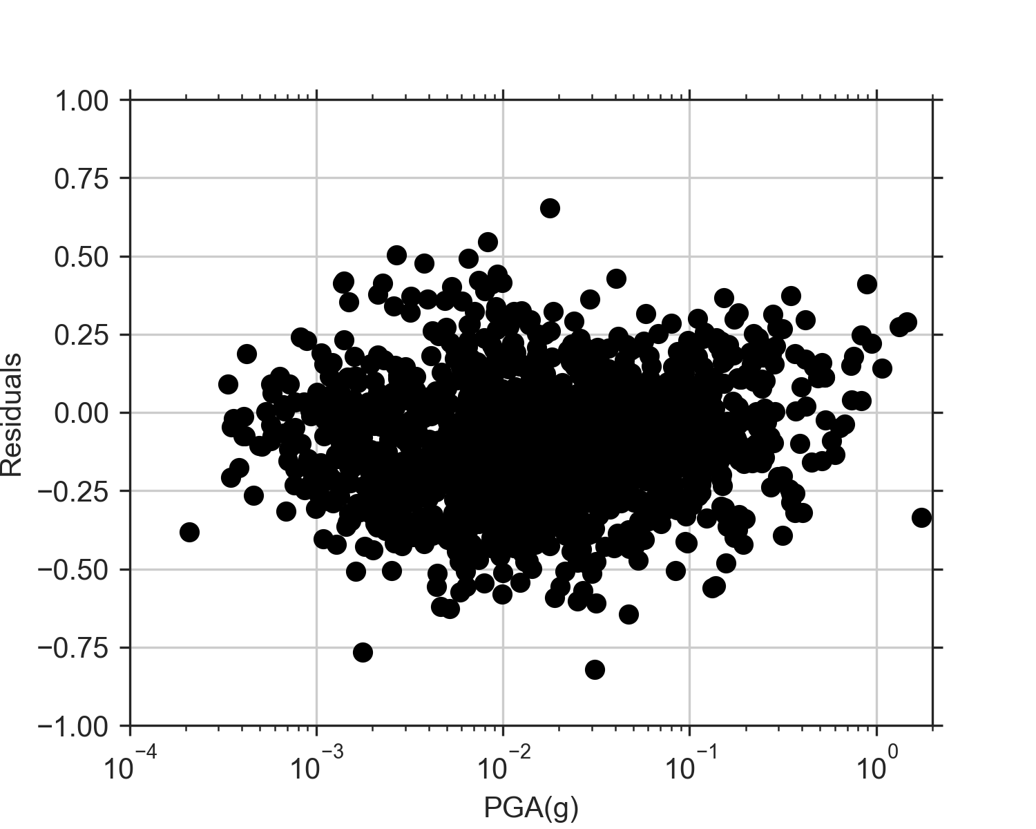

After the Liu GMPE, I worked on the one by Foulser-Piggott, which takes magnitude, Vs30, and fault distance (rrup) as the inputs. The coding of this equation was a bit more involved, and the results were not quite as promising. Plotting the predictions and the observations vs Vs30 showed decent results, but the residuals appear much greater than the ones using the Liu equation. Plotting the predictions and observations vs rrup showed strange results. The GMPE works fairly well at smaller fault distances (up to about 100km), but then the model severely overpredicts at greater distances.

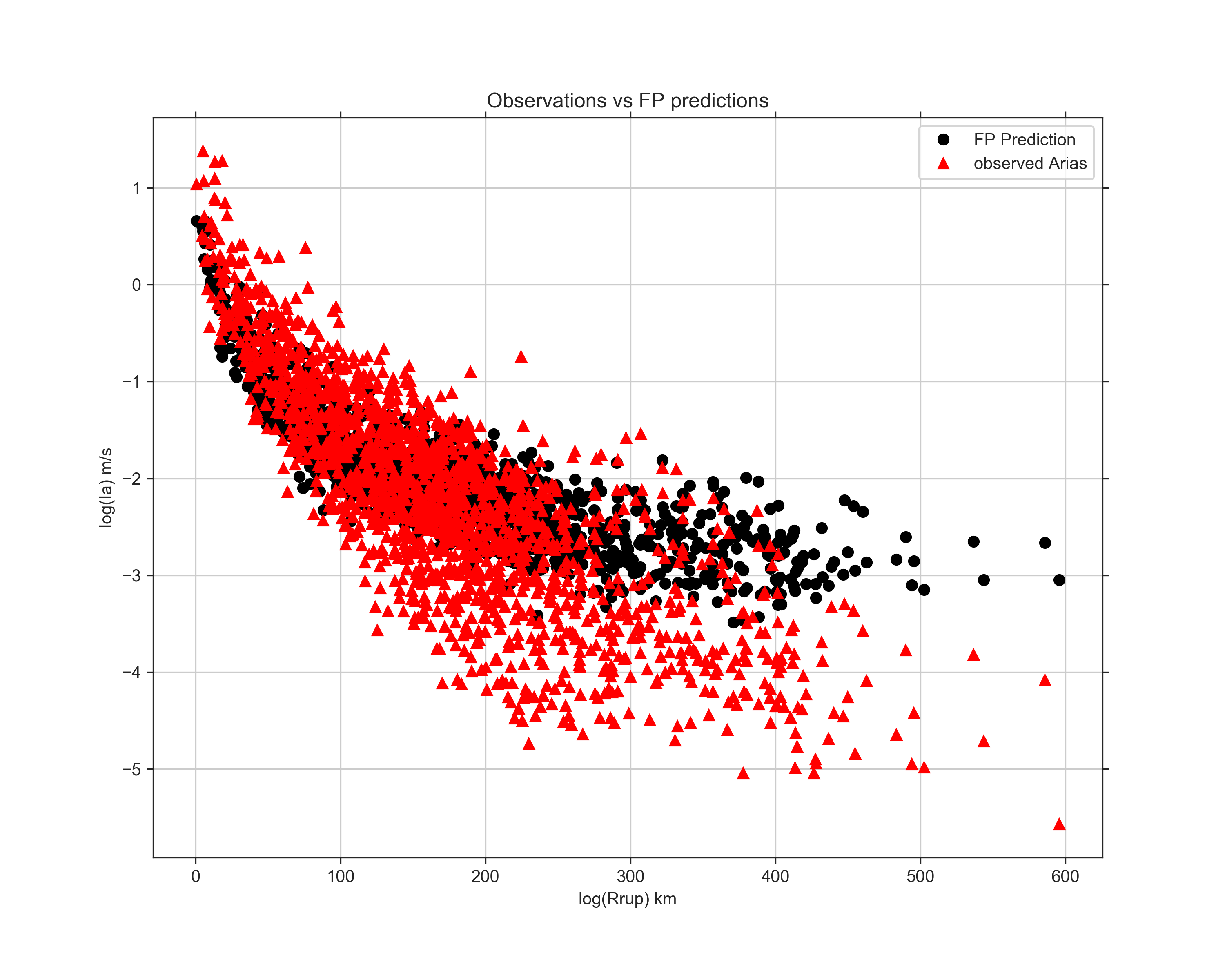
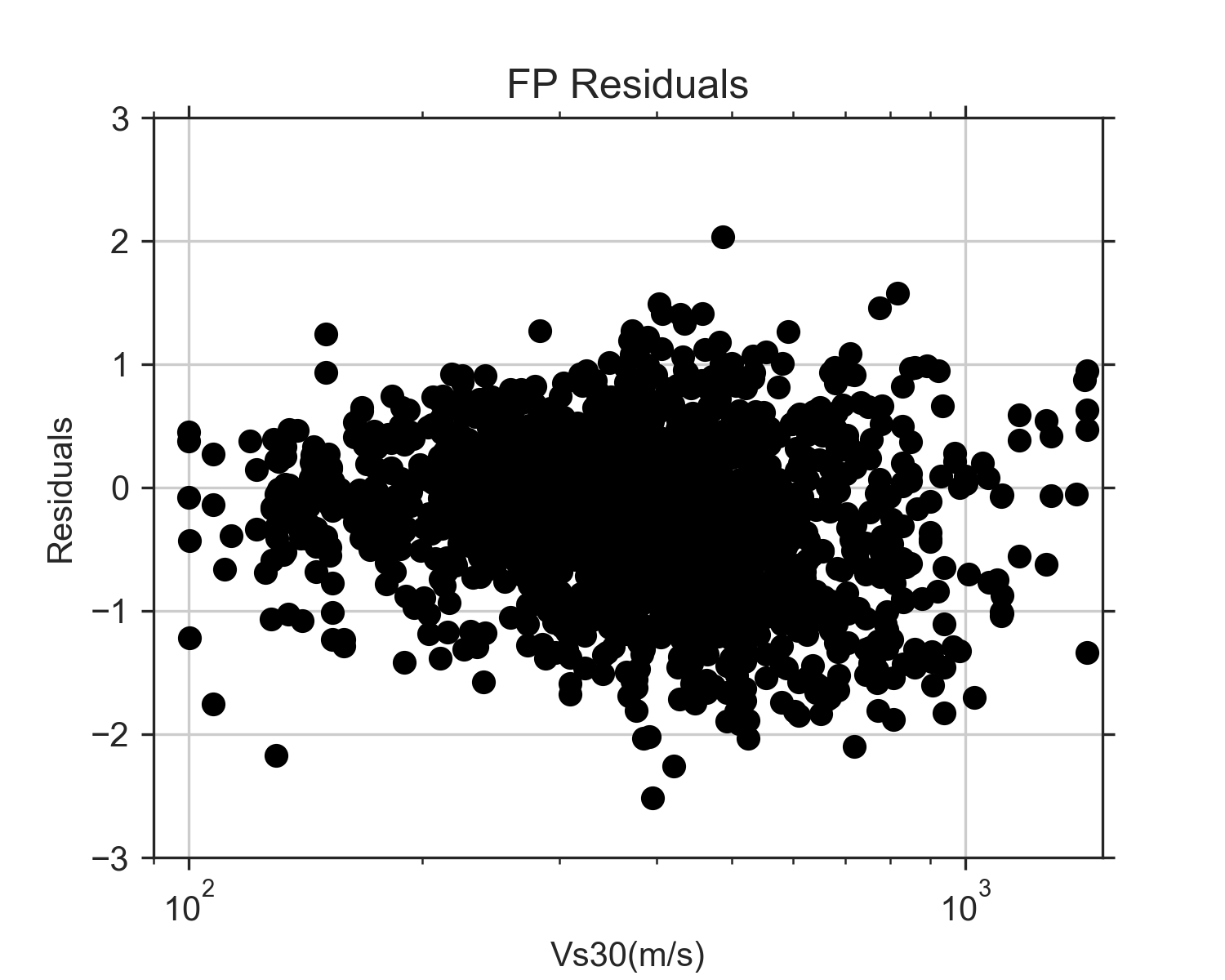
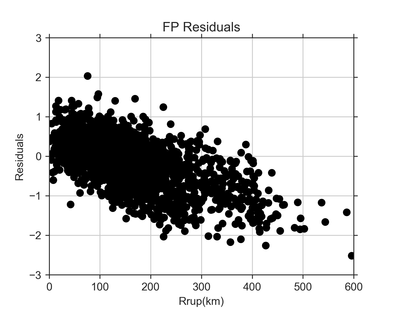
I then tried plotting the residuals but saw some strange results with these, too. The residuals vs Vs30 appeared fairly normal (flat and centered at 0), but the residuals vs reference Arias intensity (a variable calulcated in the equation), decreased a lot with ref Ia values less than 10^-2. I'm not sure why this is though. The paper showed graphs of the residuals (but for a different event), and they appeared normal when plotted agains ref Ia. I need to re-look at that part of my code next week to make sure there are not any errors. The graph of the residuals vs rrup was also unusual because they decrease greatly with fault distance. However, in the similar graph in the paper, their rrup only went up to 100 km. When I tried that, my residuals appeared to be flat. This indicates that the model works best for locations at close distances to the fault, but does not work well for great distances. I re-examined the paper, and they mention that they only used distances up to 100 km because "the aim of this paper is to produce a generic model applicable for different locations throughout the world, and, when larger rupture distances are considered, the local crustal structure can influence ground motions at the site of distance." Following these constraints, the model works ok, but a lot of our data does not fit within these constraints. The Liu GMPE appears to be much more accurate, regardless of distance from the fault.


The Travasarou GMPE can be found on OpenQuake, but I struggled to get that to work. Eric sent me an example of how to use OpenQuake, but it was still confusing, so I will have to work on this more next week. My prediction is that this code will produce less accurate results than the previous two GMPEs because Foulser-Piggot and Stafford critique the Travasarou equation in their paper, and their GMPE is supposed to be an imporvement of the Travasarou one. We'll have to wait until next week to know for sure!
Reflection
Our abstracts for AGU are due on August 1st, so I spent a lot of time this week working on mine. I went through a few drafts, but I think I finally got it where I'd like it to be. I'll admit, this was pretty difficult, especially since we don't have conclusive results yet! However, I think I was able to write a decent abstract that avoided saying what the results are and instead left it a little open-ended.
Weekend Fun
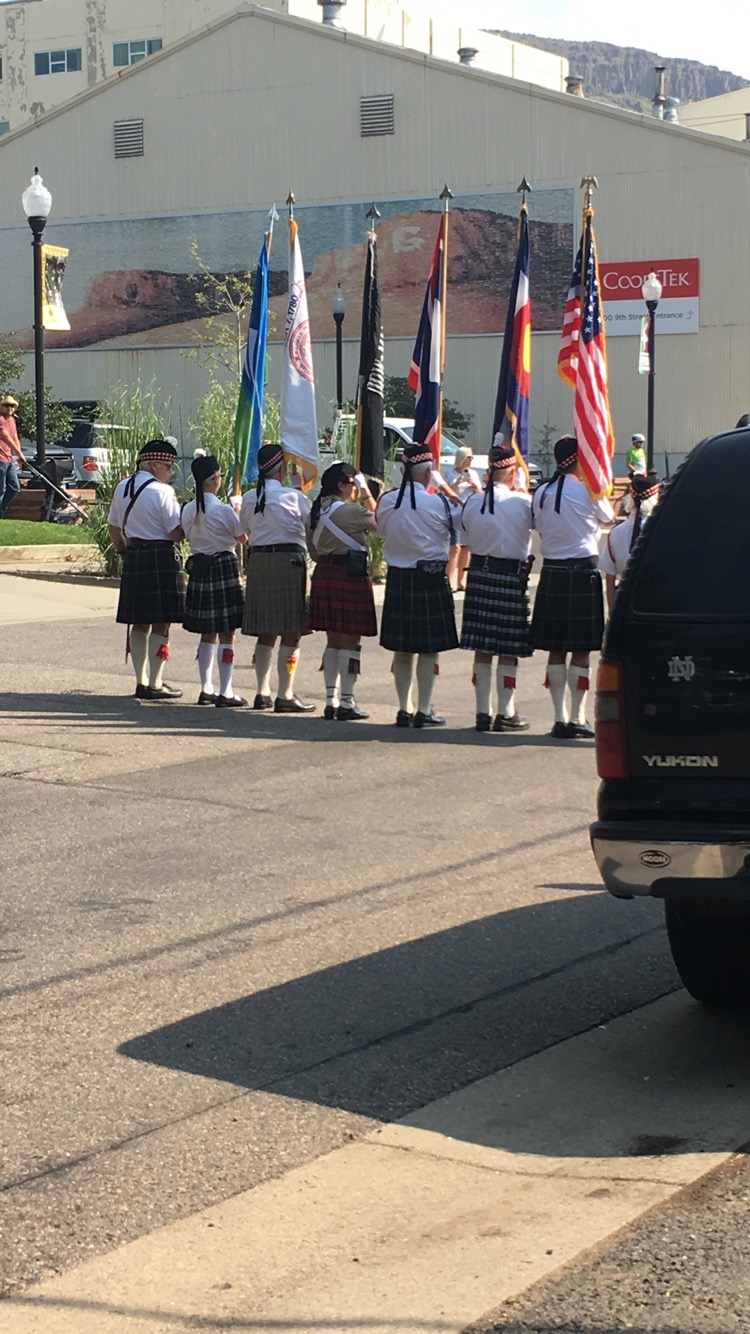
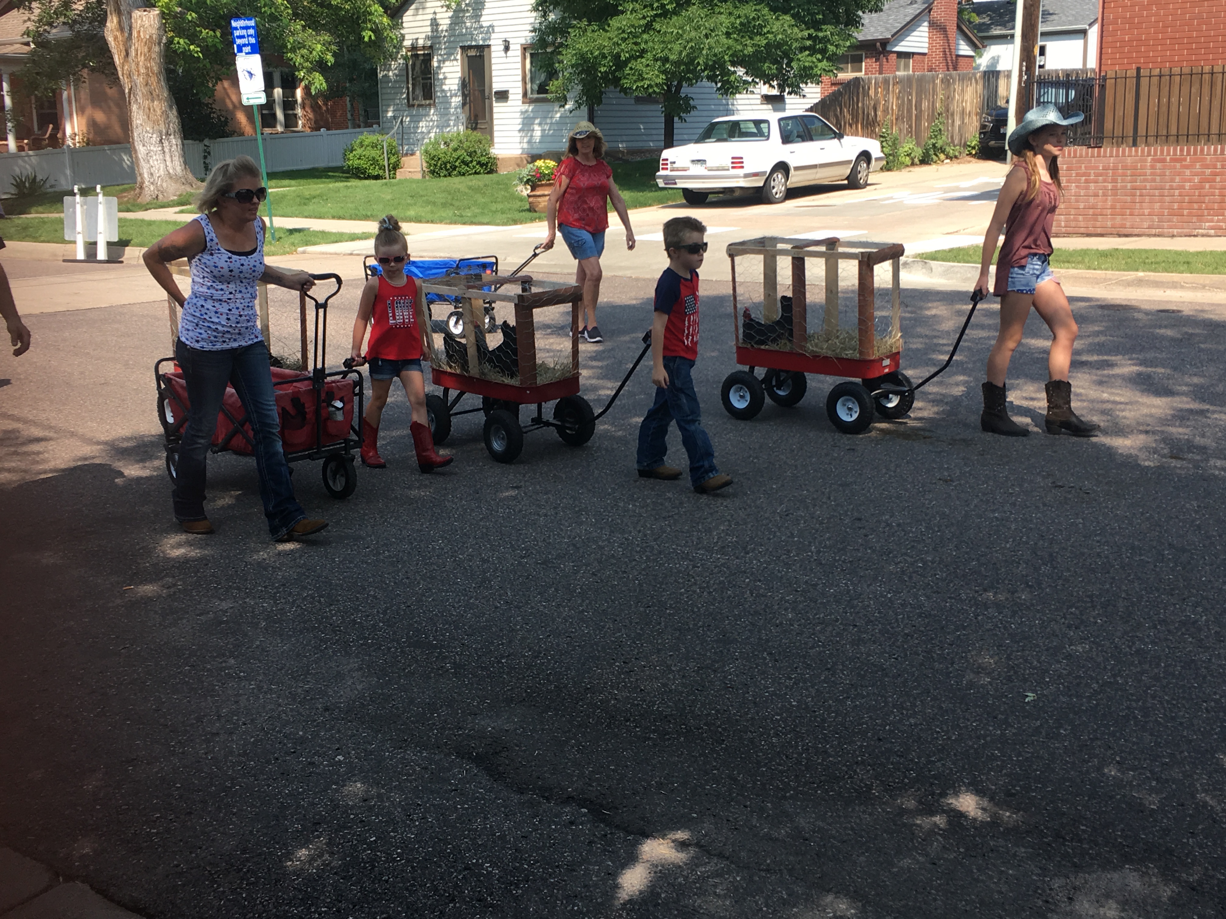
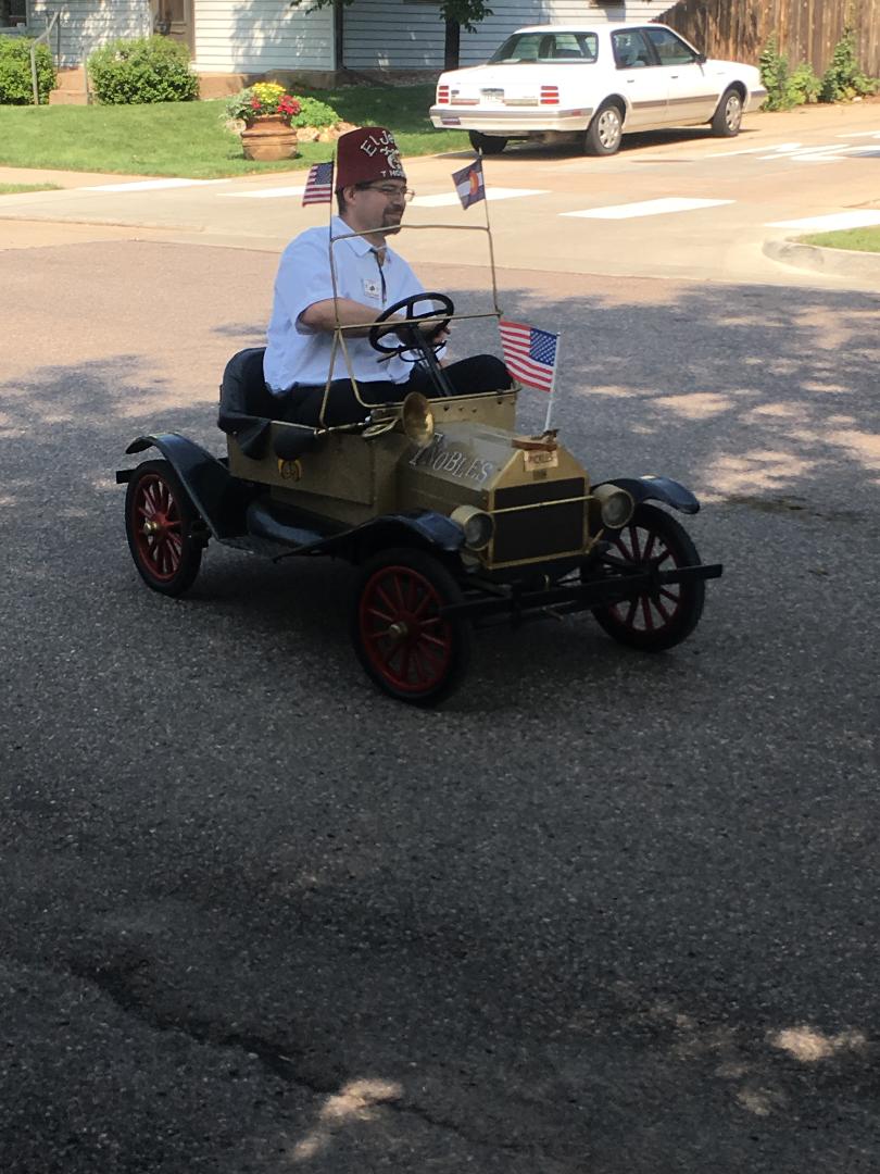
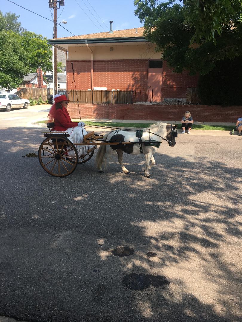
This weekend, Golden had the Buffalo Bill festival going on, which is apparently a 3-day extravaganza. I only watched the parade though, but that was pretty cool! Here are some fun pics from the parade!
Week 7: Vs30, Vs30, and more Vs30
July 23rd, 2018
Week 7
Y'all, time really does fly when you are doing something you love! I cannot believe I am already 7 weeks into this internship. That means I am 2/3 of the way through my time here! As much as I miss Utah right now, I have really grown to appreciate the beauty of Colorado.
This week at work, my main focus was to figure out how to write code to add the Vs30 values to my giant spreadsheet. As a reminder, Vs30 is the average shear-wave velocity of the upper 30 m of the crust at a specific location. We will be using these values in our ground motion prediction equations to account for site variations. Vs30 is dependent upon the physical characteristics of the location. Waves will travel much differently in a valley where there is a lot of sediment than in an area with exposed hard bedrock. This is analogous to differences in the behavior of sound waves traveling through air or water or a wooden table surface (knocking on a table with your ear on it). This week, I was able to figure out a code that would calculate Vs30 values for the kik-net stations. However, I ran into a couple of complications. Some of the stations I needed Vs30 values for did not have a kik-net velocity profile. Some other stations had profiles but had missing velocity values or 0 values. I had to edit my code to create a list of the stations without usable profiles so that we can add Vs30 values to the stations later. Although we do not have all of the velocity profiles we need, the USGS and one of my office-mates are working on creating a world map of average Vs30 values. Although these values are a little less precise, they will still be useful in our calculations. I was also able to write the code for the k-net stations but ran into similar problems with the spreadsheet not having Vs30 values for all the stations I needed. I created a list of these stations as well.
**Side note: I figured out why the k-net spreadsheet uses Vs30 values from California. For some reason in Japan, they do not have velocity profiles at the k-net stations that go down to 30 m. They only go down to 20 m, which is not useful when we need the velocity for the top 30 m. You might think that using the kik-net Vs30 values for the k-net stations might work, considering they are all in Japan. However, the kik-net stations are usually set up in much different environments than k-net stations; therefore, the Vs30 values are actually pretty different. Interestingly, sites in California are much more similar to the sites where k-net stations are set up, which is why we are using extrapolated values from California.
Getting the Vs30 values for the stations with missing data is the really hard part. I originally tried reading up on web scraping, which is where you obtain data from a website by getting information from the html script. In theory, I could write code that would access the USGS world Vs30 map website and obtain the Vs30 value from the interactive map given a set of coordinates for the station. This idea of this honestly blows my mind, but I became fascinated by it. Sadly, I could not get my code to accomplish this, and then Kate and Eric suggested a different approach. First of all, they want me to access the Vs30 map of just Japan, not the world, because it will have a higher resolution. They said I should be able to download the grid file, convert it to a GMT grid file, and then use some programs to access the Vs30 values. I struggled with this most of the day Friday but didn't get too far. I'm hoping David, the intern working on the Vs30 map, will be able to help me figure that out on Monday.
I was also able to add rake angles to my spread sheet. The rake angle is the angle of slip of an event, and it determines what type of fault it was (normal, reverse, transverse, etc...). This will also be used in our GMPEs. I didn't have to calculate anything for the rake angle because it is already on the Shakemap website for each of the 4 Japanese events I am looking at. This was basically a copy and paste task which is child's play compared to everything else I have been working on lately. I was grateful for this though! All that is left to fill out in the spread sheet are the fault distances (distance from each station to the fault). Eric has a way to calculate this and said it should only take half an hour, so we'll get that done on Monday. We have decided to use the GMPE for Arias intensity from a paper by Travasarou et al. because the code for it can be found on OpenQuake. From what I've heard, this should be pretty simple because we'll just be plugging in the values from our spreadsheet. After that, we will be able to compare the predictions for Arias intensity with the actual results to see how well the equation fits out data.
Last week, I mentioned that I started comparing geometric mean to arithmetic mean and the max horizontal component. Because geometric mean and arithmetic mean are so close in value, it doesn't seem to matter too much which once we choose to use. Most papers have been using arithmetic mean for Arias intensity, so we will probably use that one.
Reflection
These past 7 weeks have has their ups and downs, but I feel like I have overcome so much! I started this internship having absolutely no idea what I was getting myself into. I was excited, but I knew it would be a learning curve. The biggest challenge was mastering Python my work is basically centered around it. I started this internship having very little experience in coding and 0 experience in Python. Some people say the best way to learn something is be thrown right in, and boy was I! But I guess they are right, because each day my skills in coding have become more refined and I am doing things now that I never realized were possible! Some of the other challenges I have had to overcome are: figuring out how to find answers to my coding problems online, learning how to use GMT to create figures, and developing real journal-article-reading skills. I've definitely read journal articles before, but that was mostly to get a few key points I could use in a paper. However, my mentors have been asking me to read though some articles and write down any questions I have, especially in the methods. This is pretty new for me, considering I usually skim right over the methods, but it has helped me to develop a deeper understanding of what I am reading and how it can directly apply to the work I am doing.
Weekend Fun
This weekend, I decided to spend some time by the river in Golden. I sat there beatifically (GRE word) for a couple hours as I listened to the rush of the water and watched all of the families laugh and have a good time. I am currently reading a book called "Eruption," which is the story of the eruption of Mt. St Helens, so I read a couple chapters of it down by the water. I also decided to do a little work and started reading a paper called "Ground-Motion Prediction Equations for Arias Intensity, Cumulative Absolute Velocity, and Peak Incremental Ground Velocity for Rock Sites in Different Tectonic Environments" by Bullock et al. This looks like it might have some prediction equations we could use; however, it is specifically for rocky areas, and we want a more generalized equation.
My host is currently out of town for a week, so I have been home alone. I'm really not a fan of being alone at night, especially in an unfamiliar house, but at least I have a cat to keep me company! This cat loves attention, so I am currently her best friend.


Week 6: Making the Transition
July 17th, 2018
Week 6
This week has kind of been a transitioning week. Up until this point, we had been spending a lot of time gathering data, writing code to calculate Arias Intensity and CAV, and populating our data frame. However, we are now reaching the point where we will either start focusing on the rotation-independent components of acceleration and producing a paper with this, or we will start using statistics to create a model for Arias Intensity or duration that can be put into ShakeMap.
At the beginning of this week, I tried plotting Arias intensity vs distance, but was having some strange results. I realized that the way I wrote my code to integrate at specified start time did not work the way I assumed it did. I fixed this, but then ran into a new problem. I specified the "start time" to be the P-wave arrival time, which is given as a certain number of seconds after the earthquake rupture. Because our Japanese records were already processed before we downloaded them, most of our waveforms started sometime after the initial rupture. What this means is that, when we were telling it to start integrating at, for example, 6 seconds after the event, it was actually starting the integration 6 seconds after the start of the acceleration data. This cut out a lot of the data in the integration. However, with some round-about code, I was able to fix this problem as well. I plotted the ratios of Arias intensity (with a start time) to Arias intensity of the full record to see if it made a great enough difference to worry about integrating at the P-arrivals. Because the theoretical P-wave arrival times are not always accurate, I randomly chose 15 records from the usp000a1b0 event and hand-picked the P-wave arrival times. For these records (NS horizontal component), the ratio was at least 0.999. This difference is so small, and considering the fact that there is a level of error in the data and calculations, I do not believe it is worth the effort to account for P-wave arrivals. However, Kate mentioned that it could make more of a difference for a smaller magnitude event (3.5-4), so I will test that out next week. Therefore, if a window is shifted slightly due to a different start time, then some higher acceleration values could become zeroed out. I personally find this a very unreliable value to measure, but for some reason it is popular in the engineering world. Eric wants me to come up with some plots or calculations to show him how much CAVstd actually varies with the start time before he agrees to remove this Intensity measure type from our data frames.
I also started making a ton of plots for Arias intensity and the different CAVs to compare the rotational independent components. (I understand this a little better now than I did last week). Each seismic station has an orientation relative to the earthquake. If the orientation were rotated to some extent, it could change the earthquake ground acceleration values measured. Using geometric mean, arithmetic mean, or horizontal component with the greatest PGA can help account for this. These are the three components I looked at this week. From the results, it appears that geometric mean and arithmetic mean tend to be extremely close in value. The values start to become a little more spread out when comparing them to the max horizontal component, but still generally fall within 10-15% of each other. This indicates that it may not matter too much which component we choose to use in our calculations. However, next week, I will be able to use some code from another intern to calculate Arias intensity or CAV over the full range of possible degrees of rotation to see how much the minimum and maximum values differ. This might give us a better idea how much rotation or the component matters.
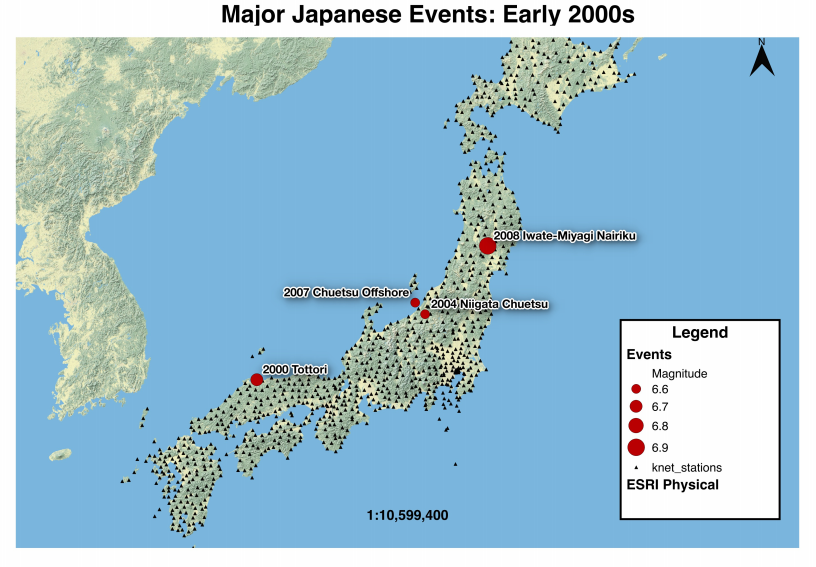
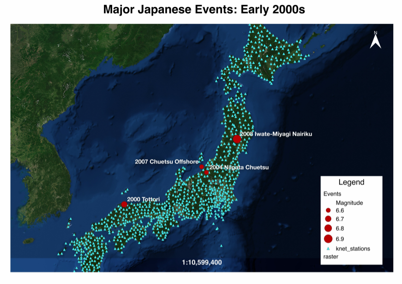
Thursday, I did not have much to do, because I was waiting on some code to be able to calculate a few things: distance from the fault, Arias intensity at different rotations, etc... so one of my fellow interns decided to take some time to help tutor me on the GMT mapping program. I was actually able to figure out the basics of it, which was pretty exciting! However, I am struggling getting GMT to work on my computer, so I still need to figure that out. I also took some time to improve the map of Japan that I made a couple weeks ago. (You can now actually see all of the knet stations!) I created 2 different versions which are shown below.
On Friday, I started working on computing Vs30 values. This is the average shear-wave (S-wave) velocity through the first 30m of the surface in a given location. I was given a folder of KIK-net station text files which lists the different velocities through the crustal layers of differing composition at each station. Calculating Vs30 itself is not too complicated. The hard part is writing the code to calculate it for each station because the stations have different layers with different depths and different velocities. This is something I am still working on figuring out. For the K-net stations, I was given a spreadhseet with the values which had been extrapolated from Vs30 values in California. I'm not sure why we have to extrapolate the K-net values rather than calculate them. (This is something I need to ask my mentors the next time I meet with them). We are using California values instead of KIK-net values for the K-net stations, despite the fact that the K-net and KIK-net stations are in the same geographic location, because a study was showed that the K-net values were much more similar to the California ones. This was discussed in a paper, which I still need to look over. Because the values are all in a spread-sheet, it shouldn't be too hard to add the K-net Vs30 values.
Reflection
This Friday, we had a webinar where most of us gave a 2-minute presentation on our projects. I actually really enjoyed this! It was easier to explain my project having two minutes this time, rather than the 1 minute for the elevator speech. However, I still felt like I needed more time to really explain any of the work I was doing. Something I have learned from these short presentations, though, is that it is super important to understand who your audience is. If they are non-scientists, a general explanation of what I am doing and why would probably be best, whereas an audience with scientific background may need less of a background and want to know more about the actual methods. This is something I will try to assess when preparing for AGU.
Fun Times
This Thursday, the other interns in my office and I went to go see Jurassic World: Fallen Kingdom. I am OBSESSED with the Jurassic Park and Jurassic World movies, and I had been dying to see this for weeks. I know it had mixed reviews, but I honestly loved this movie, and I'm so glad I didn't have to go see it alone! On Saturday, I visited the Farmer's Market again to sample a few treats, but then made my way to the sweet shop on main street. I had been craving chocolate all week, and this chocolate peanut butter ice cream waffle cone was heaven on Earth.

Week 5: Halfway Point (nearly)
July 9th, 2018
Week 5
Well, I've reached the halfway point for this internship! Technically, I have 5.5 more weeks left, but close enough, right? It's crazy how fast time flies! I feel like I've accomplished so much since I've been here, but at the same time I feel like there's so much left to do.
This week, we had the 4th of July off, and we were even given early dismissal on Tuesday, so I had a little less time than normal to get things done. One of the goals this week was to get my code for Arias intensity, CAV, and duration cleaned up and ready to be added to Amptools, a repository on Github created by some of our employees. This makes the code accessible to anyone with the link to this repository. This took a little bit of work because, when I originally wrote the code, it was for a very specific set of data. I had to edit it to work with any set of acceleration records.
I also figured out part of the issue with the PGA vs Distance graph from last week. The coordinates provided by the USGS for the event were off from the coordinates provided by the NIED (where we got the knet records) by a few degrees. This may not seem all that concerning; however, it equated to about 28 km. When I switched the coordinates to the ones from the NIED, the PGA values for the nearest stations were a bit higher, which is what should be expected.
In one of our weekly meetings this week, my mentors and I evaluated where we are currently at in the project and where we want to be by the end of my time here. Our ultimate goal is to have a model for the different intensity measures (IMs) which can be incorporated into Shakemap. However, there a few different ways this can be accomplished. To be honest, I do not remember all of our options, nor did I fully grasp what they entailed, but I do remember the basics. One of our options was to create our own ground motion prediction equation (GMPE) for these IMs. This is supposedly a complicated and potentially involved (GRE word of the week) process. We could also choose to use an existing GMPE, which is an acceptable option and definitely easier to accomplish. However, it would be best for us to create our own model if possible. There's also the option of doing a combination of the two. If I went with the easier route, I could potentially have the time to work on finding conversions between components of acceleration. I didn't quite understand what my mentors meant by this, but it would be something that could be accomplished before I leave and could produce a publishable paper. However, they said it might not be that interesting or maybe even that useful. So, now I have to decide what I personally want to accomplish by the end of my time here. Publishing a paper would look great on grad school resumes, but I would also like to aid in creating our own GMPE models. I'll have to think about it more this week.
Reflection
This week, we were asked to go over our self-reflection guides with our mentors to see how we have been progressing. I have progressed exponentially in using software to obtain data and perform data analysis. I had VERY basic training in Matlab before starting this internship and zero exerperience in Python, but I've been heavily using Python daily which has helped imporve my skills greatly. In this meeting, we were also able to see which skills we should put more focus on. I still do not feel extremely confident in figuring out the next steps in my project, producing written descriptions of my work, and critiquing work. We have decided to start discussing some papers in depth to help me gain experience critquing other people's work (which will also help me critique my own). In the past, I have read papers to look for key points that might relate to my research, but I have never really studied someone's work to figure out exactly what they did and why. Kate and Eric also suggested I start writing down in a google doc what I currently have that could be included in different parts of a paper: introduction points, methods, figures, etc... This will be helpful if I do end up writing a paper because I will have already organized a lot of the work I have done.
We were also asked to upload a figure that best reperesents where we currently are in our project. Most of the figures I have been making lately have been small plots to make sure that our data and calculations look as expected. Instead, this is a screenshot of the spreadsheet I have been making which includes event and station information for the 4 Japanese earthquakes. There are some empty columns because we have not worked with the code for those, yet.
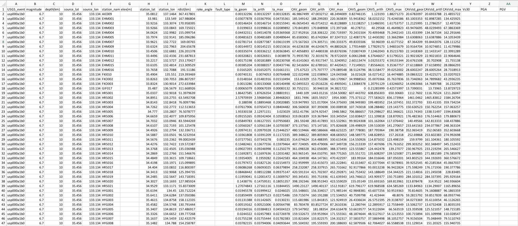
Fig 1. Portion of a spreadsheet containing event stats for the USGS events: usp00a1b0, usp000d6vk, usp000fg9t, and usp000g9h6. Knet stations with usable acceleration data were selected and included for each of the events. The data for the columns: "elev(m)," "rake_angle," "fault_type," "Vs30," "PGA," and "PGV" will be appended at a later time when code is available for these. Arias intensity is measured here in m/s and CAV is measured in cm/s.
The paper that is most central to my work this summer is probably "Ground-Motion Prediction Equations for Arias Intensity, Cumulative Absolute Velocity, and Peak Incremental Ground Velocity for Rock Sites in Different Tectonic Environments" by Bullock et al. I have examined a handful of papers, usually specifically referring to Arias intensity or CAV, but this paper sums up the intensity measures we are working with. They created GMPEs (using the maximum rotated horizontal component of acceleraion: RotD100) for these intensity measures, which they characterize as "evolutionary." This means that they are a factor of duration and frequency, which is different than previously studied "transient" measures, such as peak ground acceleration. This is critical to our application of these measures to ground failure, because ground failure is influenced more by duration than magnitude. If we decide to use existing GMPEs, this would be a great source to refer to.
Fun Times
I was invited to join my mentors and some of the other supervisors for a 4th of July party Wednesday night. We were able to see the city of Golden fireworks as well as other distance firework shows from the top of a hill. There were also a lot of storms around us that evening, which made for a pretty amazing backdrop to the show.
This weekend, I took a full-length practice GRE exam. That was pretty terrible, not gonna lie. It was incredibly long and exhausting, but it definitely gave me a good idea of where I currently stand! I also watched the second and third Jurassic Park movies to get ready for Jurassic World: Fallen Kingdom. Fun fact, all three of the Jurassic Park movies are currently on Netflix! I'm hoping to convince some of the interns in my office to go see the new movie with me next week.
Week 4: Sanity Checks
July 3rd, 2018
Week 4
I think the exhaustion finally hit this week. Every day, I just felt completely worn out physically and mentally. It must be a 4th week thing because a few of the other interns were feeling the same way. Despite this obstacle, I was able to get quite a bit accomplished this week! I started compiling all of my smaller bits of code into one program that will gather stats for each earthquake, stats for the stations recording the seismic data, and any calculations we have made so far (Arias intensity, CAV, CAV5, CAVstd) and put them into a spreadsheet. All of this information is written out into a csv file which can be opened in a text editor or excel. There are a few more things we will add to the spreadsheet (fault type, rake angle, PGA, PGV, and Vs30) once we have the code to determine those.
I also spent a good portion of this week doing "sanity checks," as one of my mentors, Eric, would say. These are things done to examine our data and make sure we are getting expected results. If anything appears out of the ordinary, it could be a result of mathematical error on our end, or it could lead us to new information in our research. One of the first things I did was use my code for Arias Intensity on a couple other sets of seismic data. In our office, many of the mentors and interns frequently refer to a geotechnical engineering textbook. This textbook gives calculated Arias intensity results for 2 stations of the Loma Prieta 1989 earthquake. I downloaded the acceleration data from COSMOS for the stations mentioned in the book, and my calculated results were almost identical!
Another sanity check I did was start looking at the compiled P-wave arrivals for the seismic stations of one earthquake event. (Reminder: we got the P-wave arrivals to finally plot at the end of last week). If the stations are sorted by distance from the earthquake source, then the P-wave arrival times should appear later with the farther stations. This is because it takes longer for the seismic waves to travel to the distant stations. However, upon looking at plots, the graphs did not appear to have this trend. Upon further looking, we realized that, although the stations were sorted, the obspy plot function would not plot them in the order specified. We then tried to use a different plotting function, but this one had all of the P-waves appearing at nearly the same time, which also did not make sense. Finally, we used a reviewData script written by my mentor, Kate, which would produce interactive waveform plots for each station and would plot the P-wave arrival times. This worked extremely well, and the P-waves appeared to "move out" with the farther stations. With this interactive program, I was also able to examine each station and remove the traces that were clipped too late. This was the case for a majority of the stations at greater distances from the epicenter. Once I deleted all of the unusable traces, I compiled all of the stations which were usable into a spreadsheet, which I then added to the code for reading in the Japanese knet files to filter out the poor data.
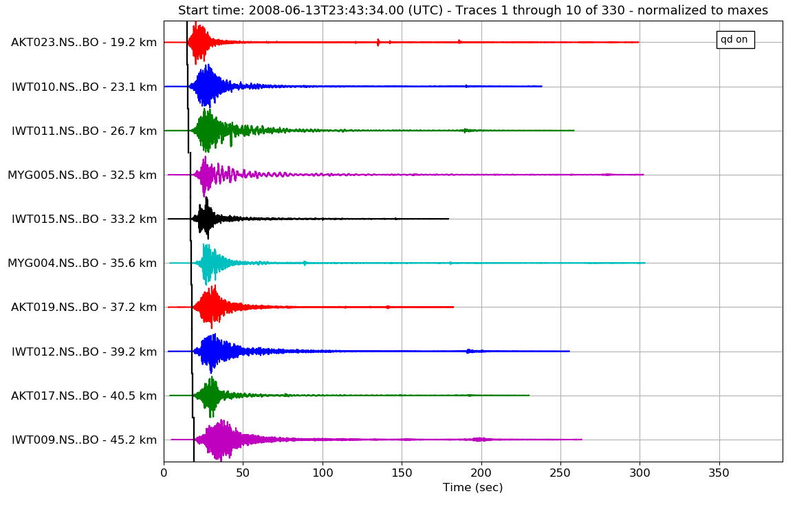
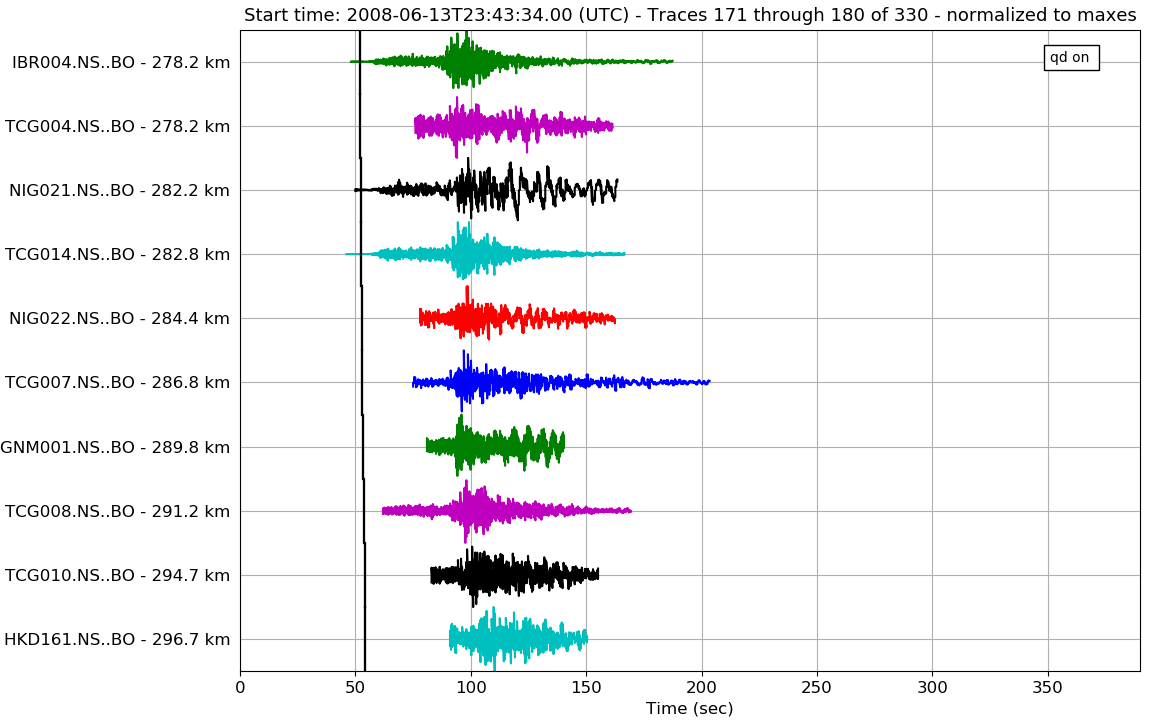
Fig 1. Snippets of the P-wave arrivals plotted on the waveforms. The arrivals are plotted as black lines. The image on the right shows some of the data that were clipped too early and had to be removed.
On Thursday, I was asked to create a kml file of the Japanese seismic stations using QGIS. This was, in a way, another sanity check. A kml file can be uploaded into Google Earth and will plot whatever is in the file. This will help us to see where certain seismic stations are located in relation to an earthquake event and will help us determine whether any small discrepancies in our arrival times and stations are of concern. If the station is located in very different terrain, the P-wave could arrive at an unexpected time. If this is not the case though, we can look back at our calculations to see if there are any minor errors.
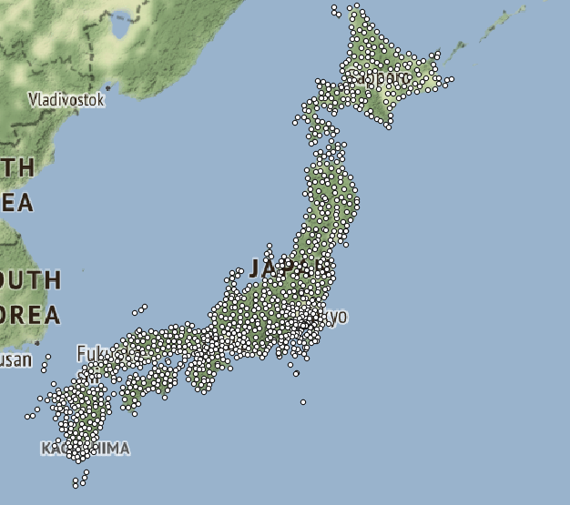
Fig 2. Image showing the coordinates of the knet stations in Japan.
One of the last sanity checks I did was create plots of PGA (peak ground acceleration) at each station vs distance from the source. This was fairly simple to do because we already had all of the distances, and the peak ground accelerations were obtained from the acceleration data. I compared my graphs with the ones provided on the website we obtained the knet data from. What is expected is for the PGA to be highest with the closer stations, and then decrease with the farther stations. This was generally the case; however, one of our plots did not quite match the one from the website. The first few PGAs were fairly small. There are some reasonable explanations for this, such as the stations being located in sandy areas or in valleys. Waves do not propagate as well though loose sediment. However, if this were the case, the plots downloaded from the website should show the same thing as the ones I created. That leads us to believe that it is an error on our part. I tried examining my data and calculations but could not find any noticeable errors. We will continue looking at this next week and will hopefully find a reason for this aberration (GRE word of the week).
Reflection
For this week, we were asked to reflect one frustration we are facing and one success we are proud of. One of the most frustrating things for me has been figuring out how to get the P-wave arrival plots to work. What's particularly exasperating is knowing that your data is correct, but you can't get the code for the plots to work as you would like them to. Python is capable of SO MANY things, and I know that I should be able to make certain ideas work, but I sometimes it takes me ages to figure out how to do so. It is also frustrating when I try to use google for help, but I just can't get the syntax quite right to elicit the types of help responses I am looking for. Despite all of this, I know that I have been able to accomplish a lot that I am proud of! The thing that I am most proud of is not one specific task, but an overall skill I have learned. When I first started here 4 weeks ago, I had very little experience in coding. Everything I attempted to write had a lot of hard-codes in it. I would type in specific values into my different lines of code to produce an answer for those specific values. However, I have learned to mostly avoid hard-coding, and write scripts that only require you to change the inputs. This makes the code much more universal and leads to fewer mistakes when applying it to different data.
This week, we were also asked to create a map of our study area. My project does not have one specific study area, but I have been focusing on a few Japanese events lately, so I decided to make a map of Japan. I originally attempted to use GMT to make the map, but I did not have the time to learn all of the idosyncrasies (you guys get two GRE words this week) of the program. The syntax of the code is quite difficult to pick up, so instead I used QGIS to make my map since I had already been working with it a little bit. In my map, I included the locations of the 4 major Japanese earthquakes we are currently working with and the locations of all the knet stations that record sesimic data from the events. The stations do not show up as well in the image as they do in QGIS (they are very small black dots). This is something I will have to edit in the future. We are studying Japan right now because it has been the location of quite a few major earthquakes and there are a lot of data to be found for those events. Once we have all of the code wrinkled out and cleaned up, we will add data from other events around the world.

Fig 3. Map of 4 Japanese earthquakes and the knet stations that recorded the events.
Weekend Fun
This weekend, I had the opportunity to go see Richard III at the Shakespeare festival at U.C. Boulder with Judy (my host) and a couple other people. It was such a fun experience! I always loved going to plays growing up, and I did a little theater myself in high school. I haven't had the chance to see one in a while, so this was pretty exciting, and it was extremely well done. Besides that, I went to the weekly farmer's market in Golden and to a church get together at our Bishop's house. I really enjoyed that because I don't get to interact with people my age too much here. It's nice that I've started making a few friends though!
Week 3: Making Progress
June 25th, 2018
Week 3
Sunday night, my account with the NIED (National Research Institue for Earth Science and Disaster Resilience) was approved! That allowed me to immediately get started started Monday on downloading the knet seismic data for 4 Japanese earthquakes: 2000 Tottori, 2004 Nigata Chuetsu, 2007 Chuetsu offshore, and 2008 Iwate Miyagi Nairiku. The data for each of these earthquakes contain hundreds of stations and the three components of acceleration (2 horizontal and 1 vertical) for each station. My first task with this data was to figure out how to organize it all...but once I figured that out, I was able to start doing calculations with it. The USGS has code for reading in knet files, so I used that to access the data. Then, I used other USGS code to combine all of the acceleration data for each station so that it was a bit more organized. With the data, I was able to calculate distance from the source to each station and the theoretical p-wave arrival times for each station. I was also able to to obtain source data (magnitude, lat lon coordinates, and depth) using a libcomcat function in python. All of this was relatively easy to calculate; the hard part came when I was trying to plot the p-wave arrival times on a vertical acceleration waveform graph. I did some searching to see if there was any simple code for this. At first I didn't find anything, so I tried to create my own code this. That did not go too well, so I refined my search and found 1 example which seemed to be exactly what I needed! Originally trying to follow the example code and not really knowing what I was doing, I used the obspy read function to read one of the files (this is important to note), and my p-wave arrival appeared to plot exactly where I needed! Once I tried looping over all of the other vertical components, my arrivals no longer plotted as expected. I could not figure out what had changed, but then my mentor looked over everything with me, and we discovered that I had used the obspy read INSTEAD of the USGS code for reading knet data. My mentor did not even realize the obspy read function could read knet data. It appeared to be working better than the code we were using though. Apparently, the Japanese stations have a weird 15 second lag which the obspy function accounts for. I rewrote my code to use the obspy read function instead, but then we ran into a few more complications. The Japanese data has been processed...kind of, meaning they had cut the data to a certain time interval, but there are some strange conversions we have to use to get the data and units into the format we need. We also discovered that some of the data was cut after the calculated p-wave arrival times. That makes those short records unusable because we are missing a good portion of the data we would need to integrate. So, our next steps are to write code that will remove the unusable data and also start working on a spreadsheet which will compile all of the data we have been gathering, such as the station information, earthquake source information, and calculations for Arias intensity, CAV, distance, etc....
Elevator Speech
Our IRIS task this week was to start working on a draft for our elevator speech. This is brief description of our projects which we could theoretically give on an elevator ride (~60 seconds). This task will help us start preparing for AGU, where we will have to present our project to numerous people from a variety of backgrounds. It will also be beneficial when trying to catch the attention of potential grad school advisors who will be attending AGU or other professionals at career fairs or interviews, who would like to know a little about the research we have been working on. Preparing a short speech can also help prepare us to explain our projects to friends, family or other random people who might want to know what our overall project is about without getting into the nitty gritty scientific detaitls. Writing mine did not take too long (probably because it was just a first draft), but I honesstly did not find it too difficult. I think that is because I have such a basic understanding of my project at the moment. It will prbably become more difficult to give a simple discription of my project once I get further into my work because I will have a deeper understanding of what it is I am actually doing and the significane of it.
Free Time
I have a fair amount of free time in the evenings, so I figured it would be a good time to start prepping for the GRE! I downloaded the Magoosh prep course (it was on sale) and have been trying to answer a few questions each night and do some lessons over the weekend. I have also been looking over vocab flashcards daily. Answering the practice questions has made me realize how unprepared I am for this test...but at least it has "galvanized" me into putting more effort into my studying! (There's your GRE word of the day)
Week 2: Coding, papers, and dinosaur tracks
June 18th, 2018
Week 2
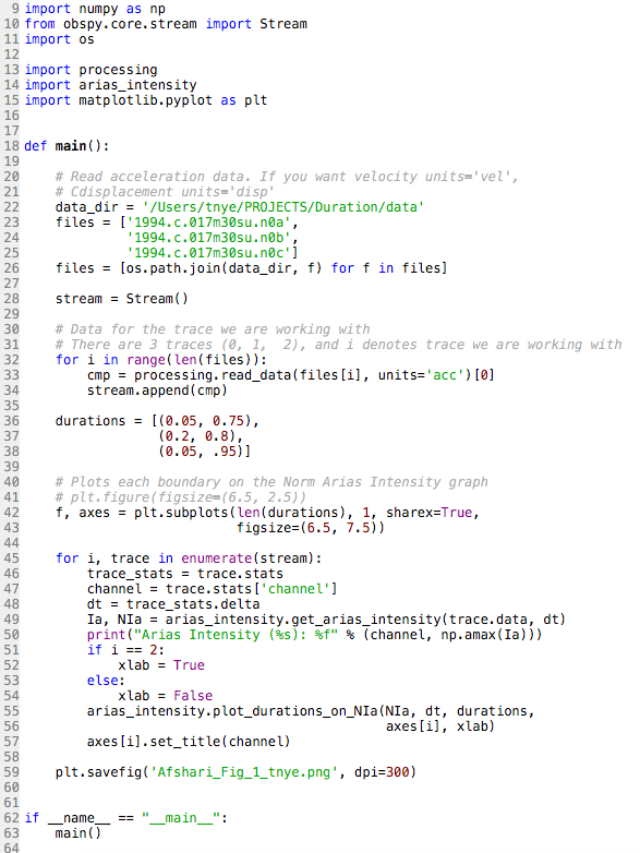
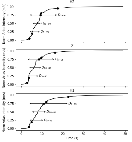
This second week of work has been a little more challenging. Putting my code into a module was suprisingly more difficult than I thought it would be. I was also still trying to figure out how to write my code in a way so that I was not hard coding everything. (Basically this means we want the code to be as universal as possible. We want to be able to type in the needed inputs for whichever dataset we choose and have the code give us the answers without having to change anything else). This was also suprisingly difficult. Nevertheless, I dug in and wrote the best darn code I could write with the help of google and stackoverflow. I was so excited to show one of my mentors what I had accomplished (probably a little too excited), but before I could explain everything I had done, he immediately started critiquing it. I was a little disheartened at first considering the amount of effort I put in, but once I swallowed my pride, I realized that the comments he gave me were extrmely constructive and will help push me to be the best at coding as I can be. Below are pictures of the finalized code I wrote for calculating Arias intensity and the figure I was able to create. The figure has three channels to represent the three components of ground acceleration: H1, Z, and H2. The H-channels are the horizontal components of acceleration and the Z-channel is the vertical component of acceleration. Although we are currently looking at all three channels, we will most likely start focusing on just the horizontal components soon.
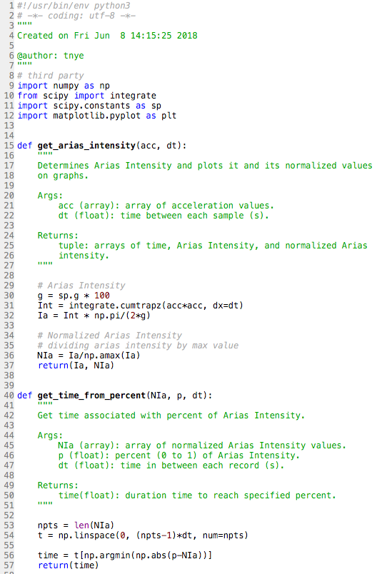
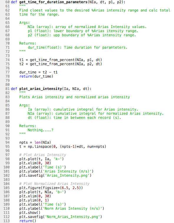

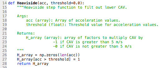
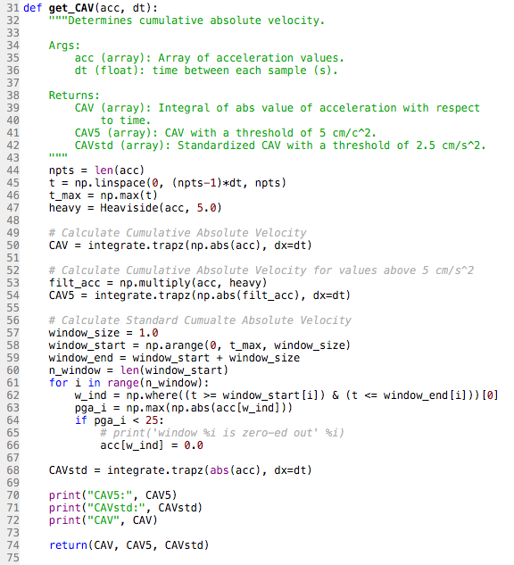
After I was able to write code to calculate Arias intensity, I was tasked with another project: write a code to calculate cumulative absolute velocity (CAV). Although the word "velocity" is in the name, we are integrating acceleraton, not velocity, to obtain CAV. It is called cumulative absolute velocity because velocity is the integral of acceleration. Because CAV is so similar to Arias intensity, wiritng the code for it was fairly easy. However, I also had to write code to calculate CAV5 and CAVstd. These are both similar to CAV, however they have threshold frequencies. CAV5 eliminates all the accelerations below 5 cm/s^2 because, for engineering purposes, accelerations below this value do not appear to cause damage to building structures. CAVstd has a threshold of 0.025 g; however, it is measured in one second non-overlapping time intervals. Originally, my mentor and I thought that 0.025 g meant 0.025 m/s^2. After reading through a paper by Campbell and Bozorgnia, we realized that it is actually the value of acceleration due to gravity (9.8 m/s^2) multiplied by 0.025. This would equate to about 25 cm/s^2. To write the code for CAV5, I had to use a heaviside function. This function would create an array of values which we either 0 for any accelerations < 5 cm/s^2 or 1 if they were at least 5 cm/s^2. This array is then multiplied by the array of accelerations. This basically zeros out any of the lower accelerations and removes them from the intergral. One of my mentors had to help write the code for CAVstd because it was a bit more complicated with the 1 second time intervals. For this, we had to create a window from 0 to our max time in increments of 1 second. Then we had to use a for loop which basically said: for the time interval, if the maximum acceleration is less than 25 cm/s^2, all of the accelerations in that interval get zeroed out. The rest of the accelerations are then integrated as with normal CAV. Below are pictures of the code we wrote for this and the resulting values for CAV, CAV5, and CAVstd. **We are still using the data from the 1994 Northridge Earthquake in these calculations**
.png)
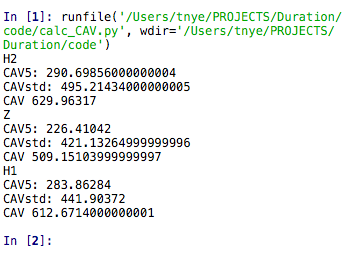
Now that we have all of this working for the Northridge earthquake data, we want to start using some data from other earthquakes. All of the data that we will be using during this internship will come from different eartquake websites. These websites have files of data that can be downloaded for specific eartquakes (acceleration, PGA, PGV, etc...). Multiple different stations record data for one earthquake, so all of the stations are listed under each earthquake. This can make the data we are obtaining a little overwhelming when there are hundreds of stations; however, the more data we obtain, the more accurate our ground motion prediction equations (GMPEs) will be. Our current focus is on the acceleration data because we can use this to calculate Arias intensity and CAV, but we plan on creating a spreadsheet which includes a variety of other data (PGA, PGV, Vs30, etc...) in the near future. The next set of earthquakes we want to look at are a couple in Japan from the early 2000s. However, I had to make an account with a Japanese server to be able to download the data, and it will take a couple days to activate my account. Hopefully, my account will be ready by Monday. With the rest of my time, I continued to read a few more papers. Here are a few things to note from the readings:
*3 factors are required for liquefaction: loose granular sediment, saturation of sediment by ground water, strong shaking
*Pore water pressure buildup depends on extent to which soil tends to densify-->related to leavel of shear strain induced in soil
*CAV5 is the best intensity measure to relate to the generation of porewater presure in potentially liquifiable soils
*CAV has significantly higher predictability than Arias intensity
**Next week, the goal is to start working with the Japenese earthquakes and also start gathering all of the different earthquake data into a spreadsheet using pandas, a programming library within python**
Papers:
"Spatial and Spectral Interpolation of Ground-Motion Intensity Measure Observations" by Worden et. al
"Ground Motion Intensity Measures for Liquefaction Hazard Evaluation" by Kramer and Mitchell
"A Ground Motion Prediction Equation for the Horizontal Component of Cumulative Absolute Velocity (CAV) Based on the PEER-NGA Strong Motion Database" by Campbell and Bozorgnia
"Ground-Motion Prediction Equations for Arias Intensity, Cumulative Absolute Velocity, and Peak Incremental Ground Velocity for Rock Sites in Different Tectonic Environments" by Bullock et. al
For this week's post, we have been asked to reflect on a skill from our mentoring rubric. One that I have been focusing on a bit this week is "figuring out the next step in a project." This skill appears to be so simple, but it is one of the most difficult parts of the research process. Knowing what our end goal is is usually pretty clear. I believe that figuring out our end goal is one of the first parts in planning out a project because it helps to guide the process. However, figuring out how to get from point A to point B can take a lot of research and creativity. I'm usually one to immediately ask what to do next before taking the time to figure it out on my own, but this week I have been trying to struggle through the process of deciding where to go next with the project. Once I have absolutely no idea what the next step should be, then I try to reach out to my mentor. This is great practice for being a real-world scientist because, one day, I will be making all of the "next step" decisions.
Weekend Fun:
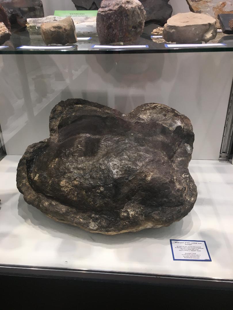
This weekend, I decided to go on a little geology hike put togehter by the Geology Museum at the school of mines. The signs along the hike described the geology of the area, explained the significance of mining in Colorado, and even pointed out some dinosaur tracks in one of the outcrops! After the hike, I stopped by the museum to check out the minerals and fossils. My favorite things on display were some small moon rock samples, a fossilized dinosaur egg, and a dinosaur track that had been filled in with mud. Later that evening, I attempted the bus system again so that I could go to a movie. However, I managed to miss the bus on the way there and on the way back, causing me to have to wait another 45 min-hour each time. One day I will get the hang of this...
Orientation and Week 1
June 10th, 2018
Hello family, friends, and any random strangers that stumble across this page! I'm Tara Nye, and I am a rising senior at Brigham Young University. I am studying geology with a minor in physics. I've been pretty busy these past two weeks, so this blog post will include Orientation Week and my first week down at the USGS.
Orientation Week
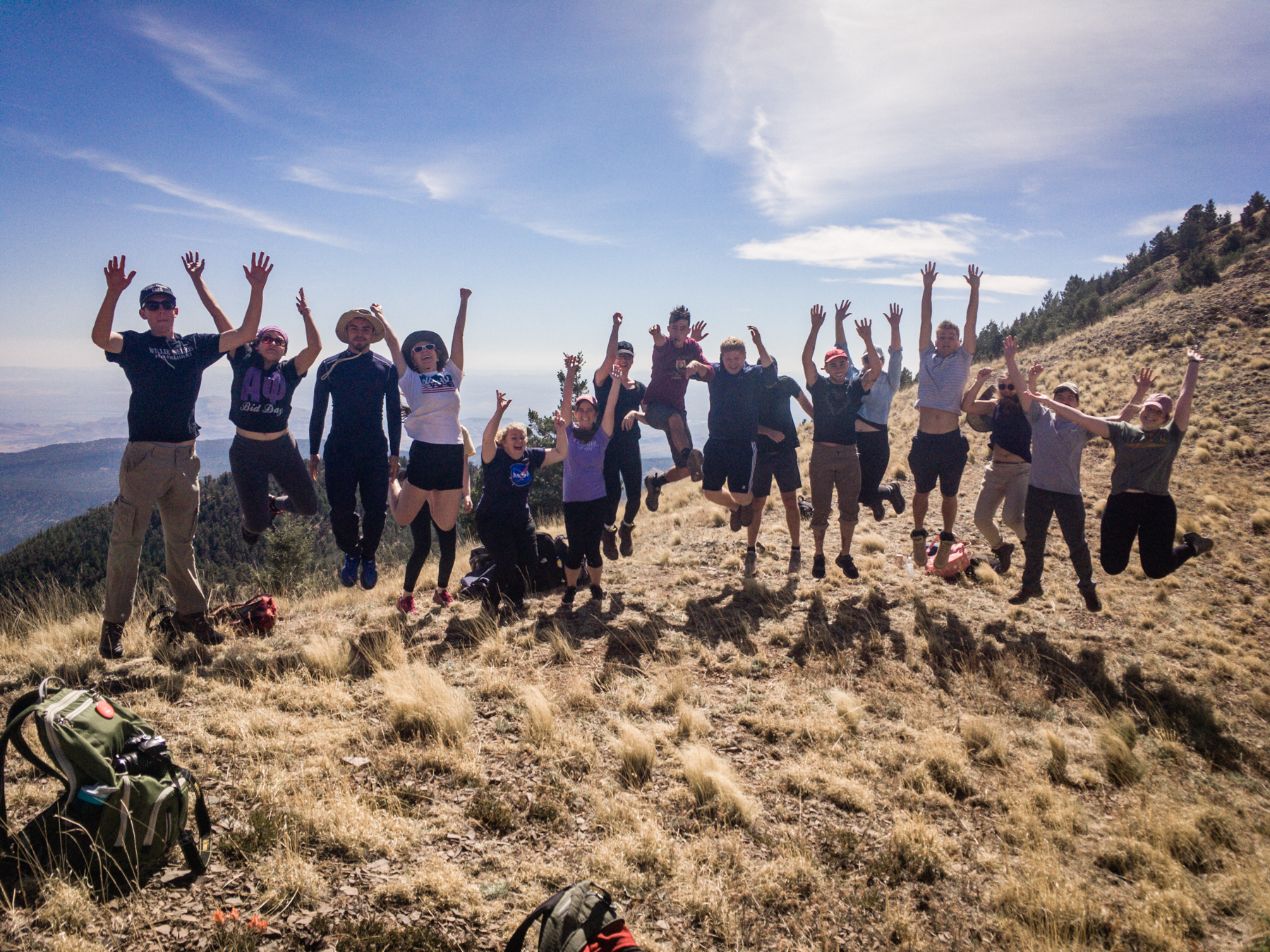
Do you ever just sit in awe at your life and think about how incredibly blessed you are? That was me on the last night of orientation week. It's amazing how close you can grow to a group of people you just met when you spend nearly every second of every day with them for a week. However, I did not feel this way at the start of the week. As excited as I was to be participating in such a prestigious internship, I was pretty terrified leaving my home in Utah and flying out to New Mexico to live with a group of strangers for a week. Like most people there, I was afraid that I would be pretty lonely. However, the first night we were together, we went out to eat as a group, and all of my fears started to dissipate. I could tell almost immediately that this was going to be an amazing week.
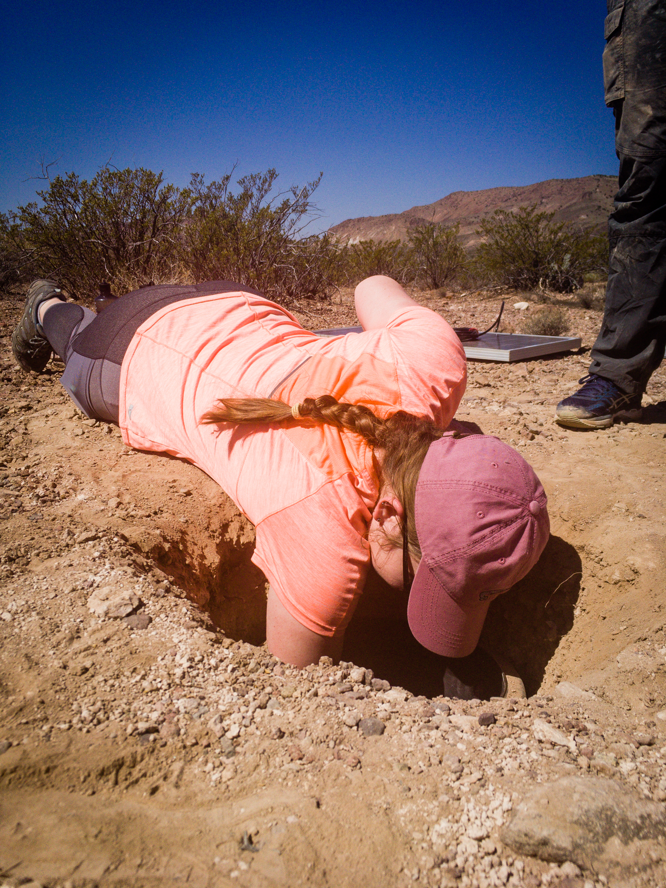
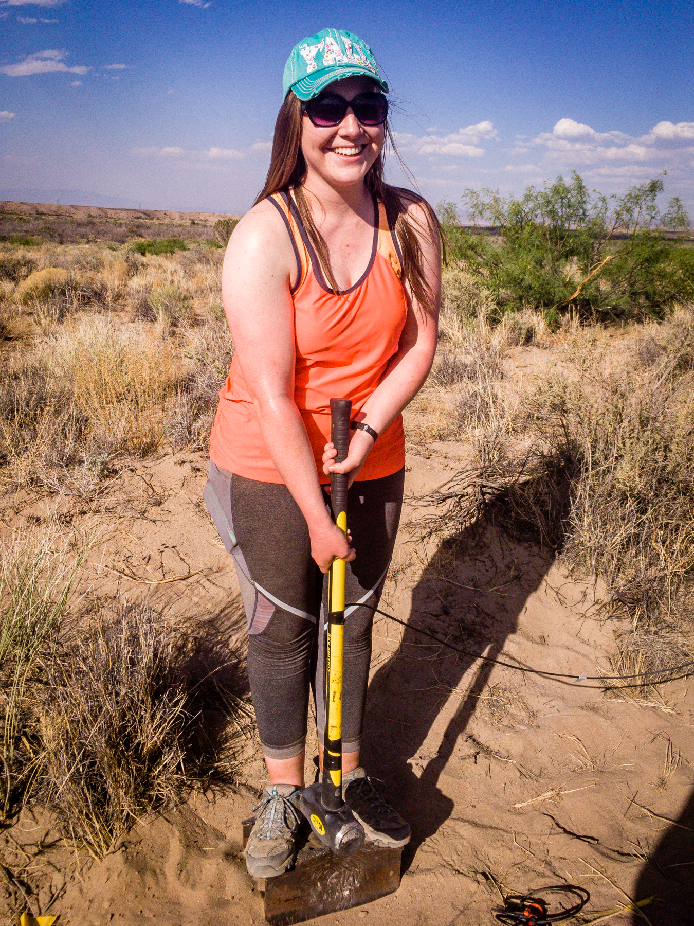
During this week, we all went through a variety of trainings in the field, in the classroom, and in the lab. In the field, we learned how to install a broadband seismoter and set up geophones for a horizontally polarized S-wave survey. We also went on a couple hikes and learned about the geology surrounding Socorro, NM. In the classroom, we had lectures ranging from seismic processing techniques, to what it's like being in different geophysical careers, to how to make the next steps after we graduate. (That last one was extrmemeley beneficial to me, because I did not realize how much I didn't know about grad school until interacting with everyone at the internship). In the lab, we learned how to navigate the UNIX system, debug matlab code, and even process some of the seismic data we collected earlier in the week. Although we did not have the opportunity to spend a ton of time on each of the trainings (there was a lot to cover), I definitely feel a lot more confident in my abilities going into the beginning of my internship.

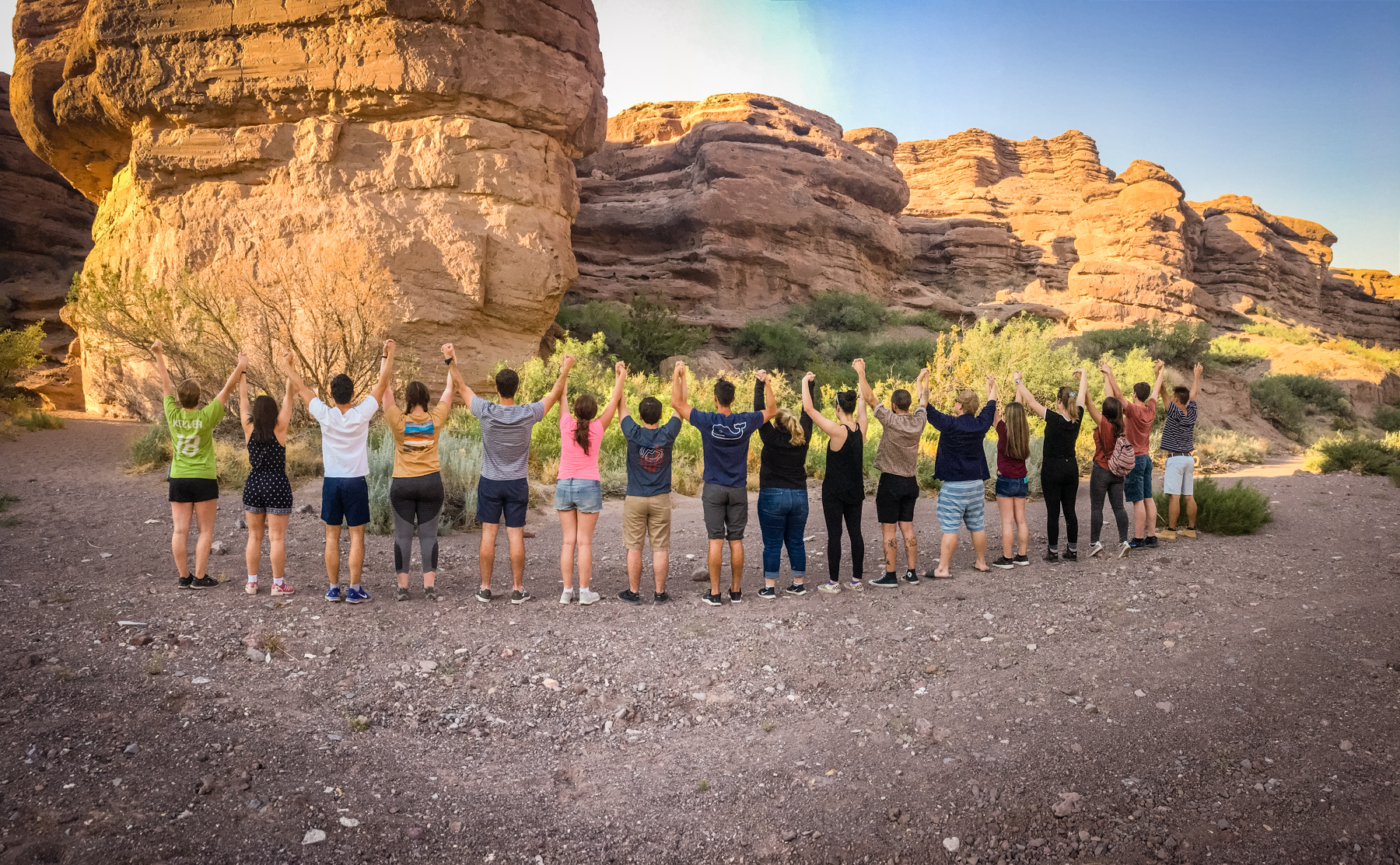
Besides all of the training, we also spent time getting to know each other. Due to a variety of blessings, IRIS was able to take on 19 students this year. (This might be the largest group they have every had). That means that I was able to gain 18 new friends! We played a variety of "icebreaker" games nightly that helped us to grow closer together. They also allowed us to address fears for our respective internships and build connections to help build us up once we are off on our own. One night, we even went to a driving range, and I learned that I absolutley suck at golf (though this was no surprise). Although we were all pretty exhausted from our 12 hour days, we still wanted to spend as much time together as possible. There were multiple nights when we would all stay up late talking or goofing off with a volleyball. (Fun fact, we are not the most athletic group of people). Throughout all of this, the catch phrase "keep it up!" was coined That just shows you what an incredibly uplifting group of people they are. On the last night, we hiked up San Lorenzo Canyon. This place is AMAZING! Once the sun began to set, we all ate dinner around an imaginary fire and gazed at the stars for what felt like forever. This was an incredible end to an incredible week.
Week 1
My first week at the USGS has been quite the experience. I am living with the dearest elderly lady and her cat, Rose, just north of the Colorado School of Mines. (This is also where my USGS office is). She obtained a masters in physics, so she has a lot of interesting life stories about being a woman in the workforce many years ago. Included in my rent are "breakfast, suppper, and laundry privileges." ***If any of you ever need a place to stay in Golden Co, I highly reccommend living with her.***
My project deals with adding duration and Arias intensity (function of the integral of squared acceleration) parameters to the ShakeMap program developed by the USGS. The purpose of this is to determine potential for landslide or liquefaction hazard due to the length of duration. The mentors I am working with at the USGS are still coming up with their best approach for calculating the duration of earthquakes, so this week was mostly spent doing background research and python tutorials. I had a little experience with matlab coming into this, but no experience with python. Therefore, when I was given the task to recreate figure 1 from a paper (link given at the bottom of this post) using the same calculations and data used in the paper, I was a little overwhelmed. However, through the help of my mentors and one of the other interns in my office, I successfully completed this before the end of the week! The figure I was asked to recreate is a normlazied (values go from 0-1 or 0-100%) graph of Arias intensity with respect to time. We obtained the acceleration data from COSMOS, a website which has a list of data from a large variety of earthquakes. The specific data we used for this figure was from the Mt. Gleason Station for the 1994 M 6.7 Northridge earthquake (the same data Afshari Stewart used in the paper). Three different duration parameters were plotted on the graph: 5-95, 5-75, and 20-30%. The time range for each of the parameters is a different value of duration. This isn't our final answer for duration, but it will help us get there. Now, I am working on putting all of the code I wrote into methods and a program (still trying to figure out what that even means). Hopefully, we will be able to use this program with data from a variety of earthquakes. My skills in python, although still extremely basic, have improved exponentially since day 1. I would consider this a successful week.
Paper I have been working with this week: "Physically Parameterized Prediction Equations for Significant Duration in Active Crustal Regions" [url=https://doi.org/10.1193/063015EQS106M ]https://doi.org/10.1193/063015EQS106M [/url];
Lessons learned this week:
1. python is your friend, not your enemy
2. obspy is python framework for processing seismic data ( I will probably use this a lot)
3. getting your ID badge from a federal center is an absolute nightmare
3. walking uphill in Golden is even harder than walking uphill in Provo (1000 ft elevation difference)
4. active shooter protection training is even weirder than you think it will be
5. Sherpa House is an amazing Indian restaurant
6. I'm in for the (geophysical) experience of a lifetime
Goals:
First Third Goals determined by Mentor:
1. Become proficient in the use of python for working with seismic data and for performing statistical analysis
2. Understand how ShakeMap works and how a new model could fir into the existing framework
3. Learn about the various ground motion parameterizations available, how they relate to ground failure triggering, and how they are computed form seismic records; choose some candidates for the model
Personal Summer Goals (Broad):
1. More experience in programmiing
2. Potential publication
3. Better idea of what a career iin geophysics/geology entails
4. Grad school networking
Personal Summer Goals (Specific):
1. Learn how to apply statistics to seismic data
2. Learn how to use python
3. Develop skills in managing my time
4. Become more efficient in reading scientific papers
5. Explore the local geology in Colorado
6. Find Grad Schools with my interests
7. Take time to prep for GRE


