Rachel Marzen

August 9th, 2013

My mentor is back! She was at a conference for the last 2-3 weeks, and so aside from email communication and some general guidance given pre-trip, I was flying pretty solo.

I learned a lot though while she was gone. Every day I would come in and work down my ever-evolving to-do list of things I thought would make the project better, and when I thought I had made an interesting comparison or obtained some meaningful result, or needed to make sure I wasn't screwing something up, I would email Gabi. Because I'd submitted my AGU abstract in early July before she left, I was very worried that because we were making interpretations part way through the analysis, that further analysis would reveal serious problems in our initial interpretations. And then my abstract would be all wrong. So while she was gone I incorporated 576 more anisotropy measurements around Hawaii, figured out how to calculate a weighted standard error, created new plots in GMT to compare the raw azimuthal anisotropy measurements to the binned azimuthal anisotropy measurements, changed my binning procedure a couple times... and on the last day before she came back I felt really tired and decided to go snorkeling.

But I completely understand why I need a mentor/advisor. Because when she came back and I met with her and her colleague Donna Blackman - walking through a stack of images I'd created to summarize the project so far - I felt like the number of great ideas to pursue and thoughtful interpretations of the data completely exploded. And articles that contained analysis that needed to be compared to our results were mentioned off-hand that I really wish I had thought to look for over my three weeks flying solo. 

So now that there's a little over a week to my internship, it's time to invert these data to change results from measurements with respect to frequency to measurements with respect to depth. And create my AGU poster. And finalize my analysis that I'm writing up in my "ResearchJournal.tex" document, which has somehow become a 30-page running list of theories and methods and results and images and explanations for why methods I decided not to use don't work. And fix some of the figures I'm created with vectors that really aren't legible - because when there's too much data on a map my solution is to make all the data smaller. If I have time, I'll figure out how to plot my inversion results just like Figure 2 of the Montelli 2004 plume article, which does a brilliant job of adding a depth perspective to a bunch of rectangular maps of seismic tomography results. And maybe re-do my weighted averaging and error calculation procedures based on some of the ideas I came up with Gabi and Donna - like nearest-neighbor smoothing that also takes into account the quality of each anisotropy measurement in the weighting process. But actually - I really just want to take this all back to school with me and keep working on it, because there's no way I can get these things finished in one week. On the bright side, with 810 measurements of azimuthal anisotropy around Hawaii - I think we have a really great final data distribution (knock on wood...) to work with - to really understand how the anisotropic structure beneath Hawaii changes with depth! And I am REALLY excited to go to AGU in December.

July 27th, 2013

... I really wish it were that simple. I realized things get complicated as I tried to draw a cartoon representation of the Hawaiian plume. I felt like I would be well-prepared for the task because once a week I get to sit around with some awesome geophysics graduate students and we talk about a couple of plume-related papers we all agreed to read. But I think that reading these papers made me realize that although mantle plumes seem simple when taught in class, they are not.

The diagram started out OK. I attached a picture of Hawaii to the surface and then I labeled the relevant layers of the Earth, like the crust and the mantle etc. 

And since we are pretty sure that the mantle flows, I wanted to add an arrow showing that flow in the asthenosphere, and had to look up some papers showing the direction of mantle flow in the near Hawaii so I could point the arrow in the right direction.

But then I started drawing the plume and things really went downhill from there. For starters, there is still a minority in the scientific community that contests the existence of plumes, and there is still some uncertainty over exactly where the bottom of the Hawaiian plume is located (e.g. Montelli et al., 2004; Foulger and Natland, 2003). However, the majority of the literature seemed to view Hawaii as a deeply-rooted mantle plume, and even as an "archetypal" mantle plume, so I decided to draw the plume as a tube of hot material rising from the core-mantle boundary (e.g. Courtillot et al., 2003). 

But I gradually realized that, in this cartoon picture, it would really be difficult to do an excellent representation of the Hawaiian plume. Factors that I decided I couldn't represent included (1) the fact that the plume probably doesn't go perfectly straight up from the core-mantle boundary to the surface, (2) the size/width of the plume probably changes with depth, (3) there is probably some significant change in the plume structure at important transition zones like the lithosphere-asthenosphere boundary, (4) mantle flow around the Hawaiian plume is more complicated than a single arrow, and convection may be layered. While I would like to draw a picture of the Hawaiian plume interacting with mantle flow that took into account all of these features, I don't think I can.

July 18th, 2013

Yesterday, I boarded the RV Sproul to witness the deployment of Ocean-Bottom Seismometers (OBS) for the first time! It was a great experience that gave me a better understanding of how the data I'm currently analyzing from the PLUME project were collected.

I was nervous because I had to be at the ship early and I had forgotten to pick up sea-sickness medication. I've never been sea-sick, but this was my first time being on a research vessel and I'd heard stories from grad students about how, the ship being small and rocking more than the bigger vessels, it was easy to get sea-sick if the weather was bad. But traffic wasn't great because people were heading to the horse races at Del Mar so I had to scrap the idea of stopping at the pharmacy so I could make it to the dock on time. 

It was a great experience. Yes - staying inside in rooms without windows wasn't so great. When we were given our briefing in a room on the ship with only a small window I kept looking at other people on the scientific crew wondering if they wanted to go back out on deck as much as I did. But I spent a lot of the day as we were traveling to and from the deployment site watching ducks, birds, and at times the cutest groups of dolphins diving in and out of the water next to the boat. 

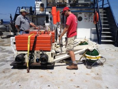
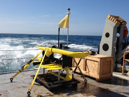
However, this was no standard OBS deployment. There were only two OBS instruments on the ship (shown below) and there was a bright yellow wave glider. I learned how to operate the A-Frame to help deploy the wave glider. From my understanding, there were two experiments running on this trip. First, they were deploying two OBS instruments but had limited the dynamic range on one of them to see how that would affect the quality of the data. Second, they were working on a project to get real-time data from ocean-bottom seismometers. 

Usually, the data from ocean-bottom seismometers are only retrieved when the instruments are retrieved. If someone is interested in data to analyze a specific event - such as a recent earthquake - they would need to wait several months until instrument retrieval for seismic data from the oceans. With the OBS-wave glider apparatus (which I was told were ~$250 thousand each to build), the OBS can communicate at a specific frequency with the wave glider circling above the instrument. The wave glider is powered by solar energy, uses the energy of wave motion to move, and adjusts a rudder to steer. 

I also talked to the captain on the ship as we were on the return trip. I asked him what tools he was working with, and was pleasantly surprised when he told me to sit in his seat (which has a fantastic view) as he described every instrument he was working with in order to steer the boat. He was able to take this time to explain things to me because he had set the ship to automatically travel on a bearing oriented towards Point Loma. In addition to multiple compasses and steering equipment, he had a computer that showed water depths and could provide the bearing from the ship's current location to another selected location, radar and other tools to detect nearby ships, and data on sea-floor depth directly beneath the ship from the ship sending down and receiving signals. Right after his grand tour of the captain's area, we saw a school of dolphins swimming right next to the ship!

I'm so glad that there were members of the scientific party who took the time when I asked questions to explain things like how the boat operated, how the instruments were designed, and what processes they were running - such as triangulating the location of the OBS's and monitoring the path of the glider in a ~500 m radius circle around the OBS, and other seismology-related projects they were working on. 

July 16th, 2013

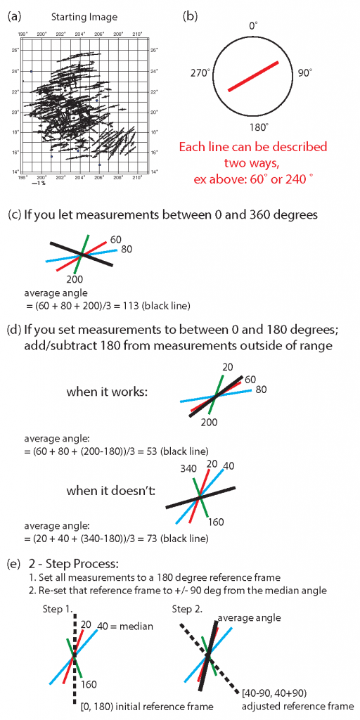
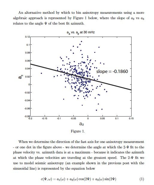
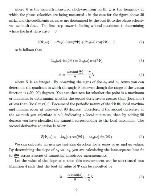
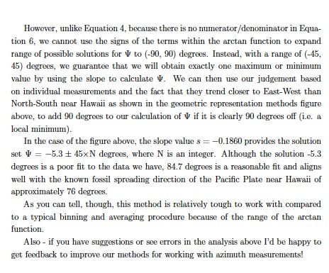
An interesting problem I was working with when designing methods to bin and average our anisotropy data into a grid format stemmed from the fast-axis calculations: the range of the arctan function, and the fact that each trend representing the fast axis orientation can be described by two angles over azimuth range [0,360]. Gabi and I thought through two approaches to this problem. However, because the first approach is best explained by visuals, and the second approach requires a combination of visuals and equations, it's a little unorthodox but the rest of this blog entry will be shown or described in the following figures. Also - this is a work in progress. If you have interesting suggestions or see an error in logic, I'd be happy to hear about it and make adjustments to my current set of calculations (which is based on the geometric explanation below). 

Approach 1:

Approach 2: 

July 8th, 2013

Happy (belated) 4th of July! After spending the weekend at the beach in LA, I'm ready to get back to business. 

Three updates on the project:

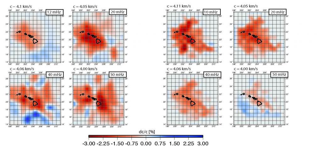
1. A comparison of the first term of the 2-Psi fit data I have collected compare well with the data from Laske et al. (2011), in which measurements of shear velocity are also made but with a different method (2-station path-averaged dispersion curves), which makes us more confident that these recent results are a good representation of the velocity structure beneath Hawaii. Below is an image showing results from the method of Laske et al. (left), and the results I have obtained so far (right). Phase velocity anomalies (%) are measured relative to Nishimura & Forsyth (1989) velocity values for Pacific plate between 52 and 110 Myr, where red is slow and blue is fast. I hope you feel the patriotic spirit behind these plots! These plots may improve as we try to incorporate the differential pressure guage data from the SWELL pilot experiment and from Phase 1 of the the PLUME project to get better resultion close to the Islands.

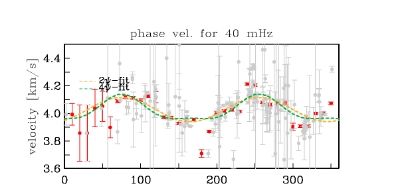
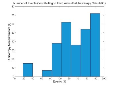
2. After looking through the results from various combinations of land/OBS data, my mentor and I have decided to discard the data from the land stations, but counter-balance the resulting decrease in geographic coverage of azimuthal anisotropy measurements by expanding the tolerance of triangle size to an average side length between 1 and 7 degrees. The result will be a decrease in resolution, especially in areas to the northeast where there aren't many smaller triangles that provide azimuthal anisotropy measurements over a smaller area. I have generated 284 anisotropy measurements, for which there are typically 80-180 events contributing to the 2-Psi fit, to plot changes in azimuthal anisotropy in an ~13x13 grid around Hawaii. Below I show an image of a histogram of the number of events contributing to each anisotropy measurement, and a sample of how the 2-Psi (yellow line) fit to the event data (grey = raw data, red = binned data) are used to determine the direction of the fast axis (the azimuth corresponding to a local maximum in phase velocity) and the amount of anisotropy (%).

Now I'm working on using the data from the 2-Psi fit of the phase velocities of azimuthal anisotropy to generate a map that shows how azimuthal anisotropy changes with frequency both in magnitude and direction. Because there are so many measurements, I plan on binning and averaging the fast-axis directions after setting them all within a 180-degree range, and plotting those over a smoothed grid of binned/averaged % anisotropy measurements. I'm currently not sure the best way to plot line segments representing the direction of anisotropy based on azimuth, but looking through the manual it seems like tilted thin rectangles may be a good bet. Vectors may be good as well except I don't want to get an arrowhead because that wouldn't be representative of the fast-axis measurement. I'm open to GMT suggestions!

3. Now that we have made these measurements, I think we will be starting the inversion to measure azimuthal anisotropy with respect to depth (from our measurements based on frequency) soon!

June 25th, 2013

In my last few posts all my titles corresponded to names of songs... but since I wanted to talk about the methods I was using in my research I couldn't think of a song off the top of my head that would be appropriate. But no fear! A quick google search revealed that there is actually a band called Tool (http://en.wikipedia.org/wiki/Tool_(band)) so I am able to keep the music-related titles going!

Now that I'm fully submerged in the data analysis aspect of my research (although I still frequently have to reference textbooks and articles to understand why I'm telling the computer to do the things I do), I can describe what tools I'm using to calculate the seismic anisotropy of Rayleigh Waves.

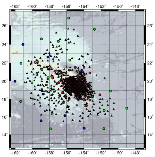
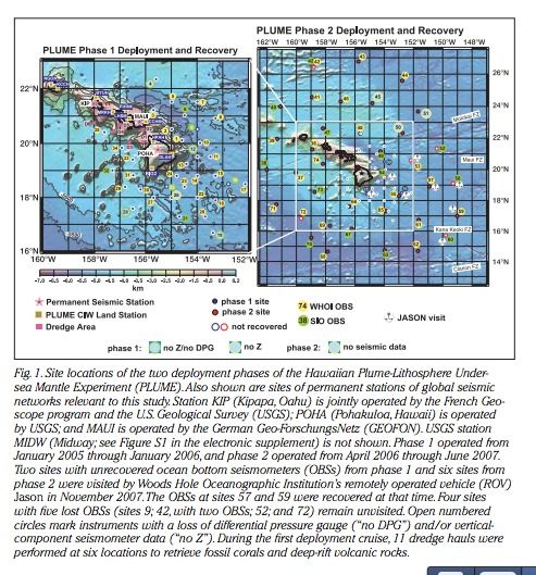
First: the data. I'm combining data from the second phase of the PLUME deployment where 37 OBS stations were placed around Hawaii at a spacing of ~200 km with data from land stations. Hopefully, this pool of data will expand to include data from the earlier SWELL pilot experiment and data from the first phase of the PLUME project, where 35 OBS were placed more densely and closer to Hawaii. Complicating this process is the fact that the instruments had different levels of success at collecting seismic data, ranging from having no data to getting over a year's worth. Additionally, because we don't know the instrument response of the SIO OBS, they have to be analyzed separately from the WHOI OBS and land stations. This image from my mentor's article in Eos Transactions (Laske et al., 2009), shows the locations of the stations and which did and did not provide data.

Second: the analysis. My mentor largely programs in Fortran. I was largely trained on Matlab. So what tends to happen is that when I write the script it's in Matlab, and if my mentor writes the script it's in Fortran. I do most of my analysis by running the Fortran executables through the terminal and writing small scripts such as with awk that automate the process so it's faster and I can do something else while the analysis is running - like read or blog here. I use my Matlab scripts to figure out, with a given station configuration, on which data to run the Fortran executables. I then use GMT to plot the results, and modify the GMT scripts depending on the data I'm plotting and what I am trying to show.

Then I look through the outputs of these processes and identify how to modify the analysis to improve the results. For example, I went through the 309 azimuthal anisotropy measurements yesterday, which were very messy, and identified ~200 for which the trigonometric fit was not a good fit for the data, generally because (1) there weren't enough data, (2) the data were messy, (3) there were some relatively anomalous points with small error bars that skewed the fit - although my mentor set a minimum error threshold so this is less of a problem, or (4) some combination of the problems above. I re-made the anisotropy maps with the better ~100 measurements. Today, I'm going to run my scripts to determine more station triangle combinations to fill in the southern portion of the Hawaiian swell, where data were lacking in the last analysis.

June 19th, 2013

I chose this title above because parts of my research this summer - while very meaningful - involves plugging data into a script and evaluating whether the results are reasonable. A lot of the early-stage work involved in my project has already been completed - so it's likely I won't be seeing the original seismic data during my analysis this summer.  I hope to gradually learn what other people did to process the original data, though, and to better understand the dataset I've been handed to analyze.
My current task is to run scripts that calculate the azimuthal anisotropy of Rayleigh waves around the Hawaiian Plume at various frequencies (where lower frequencies sample deeper). Although a lot of research has already been published about the Hawaiian Plume data including various forms of tomography and receiver functions, this analysis will be the first to show how anisotropy might change with depth.

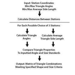
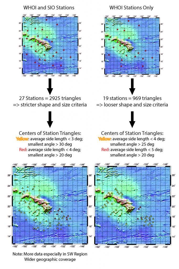
My most recent idea was to maximize the number of anisotropy measurements we could obtain from the data available. Measurements are made by comparing arrivals across a triangle of three stations. From talking to my mentor and looking a previous data - I approximated size and shape contraints for "good" station triangles (closer to equilateral, not too small or big) and designed a script that would output every 3-station combination that met the criteria - rather than eyeballing like in the past. The general algorithm is outlined in the flowchart:
I was really excited at first because I was initially working with a station list that included extra stations whose data we can't actually use because we don't know the instrument response - so I was getting well over 50 triangles even with somewhat stringent size and shape criteria (all angles between 30-120 degrees, average side length 0.5-3 degrees). Later when I removed the Scripps stations we weren't using, the picture below shows the sad effect this realization had on the number of good triangles that could be used to calculate anisotropy across the region.

Perhaps the data from land stations can be added, or SIO instruments can be compared to one another time permitting. For now though, the figure on the bottom right illustrates the 36 yellow (from criteria applied to all stations) and 7 red (from more liberal criteria applied to NE stations because of otherwise sparse sampling) station triangles that I will be analyzing over the next few days.

Overall, though, I'm really optimistic about the effects this method of determining station triangles will have on the analysis, as it imposes more consistent quality constraints while providing more combinations of triangles than had been determined manually in the past.

June 14th, 2013

Public transportation is apparently pretty terrible in San Diego. So my twin and I packed our bags in the car to drive cross-country (Virginia to California in 6 days!), building in some time to see landmarks along the way. We stopped in Nashville and binged on fried food (because Steph vetoed touring the Grand Ole Opry), confirmed that there really wasn't much to see in Arkansas, perfected our hotel-finding skills, and visited the Grand Canyon. 

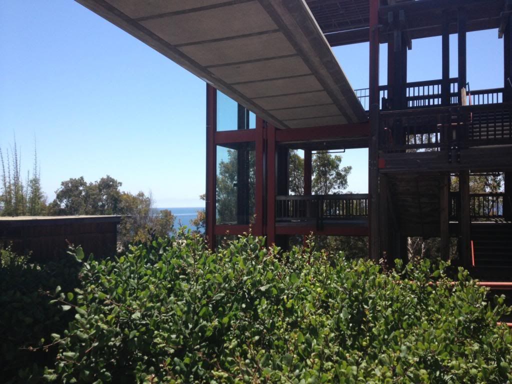
I am very excited for my project this summer, and working with Gabi. I've been spending the last week doing background reading to start writing about my research, meeting graduate students and other faculty members, seeing a PhD thesis defense for the first time, and learning when to call a car mechanic (when it sounds like you're dragging a trash can behind you as you drive). Also, SIO is gorgeous. I can't believe that I'm working in a building that is walking distance from the beach, with an aquarium up the hill and oodles of geoscientists everywhere. I'm posting a picture here, and you can see the ocean in the background. 

Goals I have for this summer include:

(1) Learning about new methods related to performing seismology research, and eventually understanding them and why they work

(2) Keeping an updated journal of my research in Latex - which I've wanted to learn for a while

(3) Meeting other students and learning about their research, so I'll make friends and have a better idea of what I may want to study in graduate school

By the end of this summer, I hope to understand my area of research - the Hawaiian plume - and the methods that I have been using to analyze the PLUME project data, well enough so that even if I don't get the results I hope for now by the end of 10 weeks, I will have some idea of how to improve data analysis for the future, and how the results I have achieved relate to other studies and previous results.

But for now, I'm just really excited to be in San Diego, spending the day learning about Hawaii, and getting to know my mentor and the culture at Scripps.

May 30th, 2013

Hey Y'all!

I'm in the middle of orientation week right now. It's awesome being surrounded by so many people who love geophysics and seismology as much as I do! 

One of the great opportunities I have had this week is learning how to install a seismometer. It was hot outside and my luggage was left in Chicago so i was in flip flops and a skirt, but I still had a lot of fun. Alexis and I set up the solar panel really quickly, so then we got to help with burying the equipment -- bare feet are surprisingly helpful at filling a hole with sand.

Setting up the seismometer helped me understand the many issues that can arise when collecting data - including the effects of changing temperatures, incomplete burial, etc. I think this experience will help me when I go to Scripps and analyze OBS data, because there are many more complications that can arise when collecting seismic data from instruments that are thousands of meters below the surface.

We only have a few more days left here in New Mexico, but this experience is leaving me very excited for my research this summer!