by Dr. Alka Tripathy-Lang and Dr. Wendy Bohon
More than 150 kilometers east of the San Andreas Fault, the small town of Ridgecrest, California, was rattled by a magnitude 6.4 earthquake on July 4, 2019. 34 hours later, a magnitude 7.1 earthquake ruptured approximately 10 kilometers away from the initial shock. The rumblings of this quake were felt through much of southern California, and parts of Arizona and Nevada. Called the Ridgecrest earthquake sequence, more than 111,000 earthquakes greater than magnitude 0.5 occurred during the first 21 days, including 70 events greater than magnitude 4. Fortunately, this area is sparsely populated compared to coastal California. Damage was limited to the Mojave Desert towns of Trona and Ridgecrest, as well as the Naval Air Weapons Station at China Lake, whose facilities sustained major damage.
The 1999 magnitude 7.1 Hector Mine earthquake was the last major event in the region, occurring in an even more remote part of the Mojave Desert. Since then, earthquake monitoring has significantly improved. The Southern California Seismic Network, comprising 400 seismic stations, has nearly doubled in size. GPS stations are installed throughout Southern California. High resolution spaced-based remote sensing methods, like InSAR, determine how the ground moved relative to the satellite, and can be deployed very quickly after an earthquake.
For scientists who study earthquakes like Zachary Ross, a seismologist at Caltech, this earthquake sequence provided a rare opportunity to study how large earthquakes unfold. In a paper recently published in Science, Ross and his colleagues’ analysis of seismic and geodetic data reveal how this earthquake sequence evolved on unmapped faults oriented orthogonally to one another. Faults range between 1 to more than 10 kilometers in length, with the largest shocks rupturing multiple faults. Only a few years ago, these types of multi-fault ruptures were considered unlikely, underscoring the importance of Ross and colleagues’ work. Furthermore, the cumulative length of the newly formed fault zone extends more than 75 kilometers, stopping just short of another major regional structure—the Garlock fault.
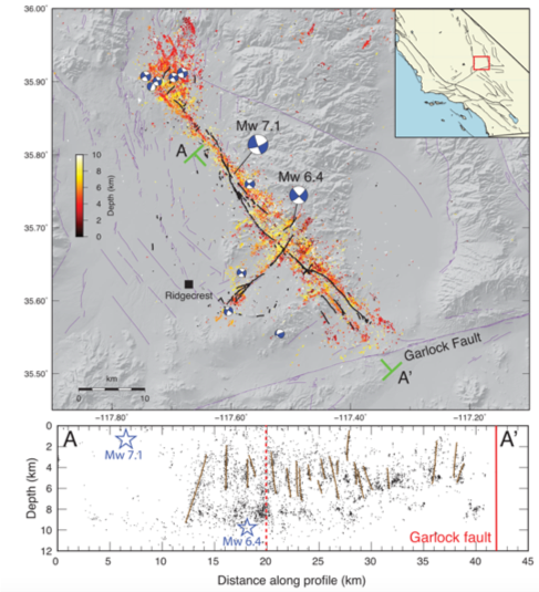 An earthquake’s hypocenter prescribes where it nucleated in the subsurface. By plotting the hypocenters of many regional events in three dimensions, seismologists infer how faults are oriented below our feet (Figure 1). However, Ross cautions that this process isn’t as simple as it may seem. Though determining the precise hypocenter is difficult, the factors that complicate standard location methods can be overcome by relative relocation, which Ross says, “is a separate process that is performed on a collection of nearby events.”
When relocating earthquakes near one another, Ross explains, the relative timing difference between two events on a seismogram arise entirely from differences in the earthquakes’ hypocenters. But instead of looking at only two events, Ross and colleagues used 111,918 quakes that occurred during the Ridgecrest earthquake sequence. With data from various sources including the IRIS DMC, they successfully relocated 46,512 events to within ~100 meters horizontally and 350 meters vertically, relative to one another (Figure 1). These results laid bare the complex nature of the earthquake sequence, with numerous faults rupturing at right angles to the main fault. Put another way, the dominant trend of the fault is northwest-southeast, but many subsidiary faults that ruptured near-simultaneously trend in the opposite direction.
To see how the ground moved as a result of the earthquake sequence, Ross and his colleagues turned to InSAR satellite data. By comparing before and after images, they can see where the ground broke. Typically, interpreting InSAR data involves counting color fringes on either side of a fault. Coupled with how these colors progress through the rainbow, scientists can calculate how much the ground moved up or down relative to the satellite (Figure 2a). At Ridgecrest, near many of the faults, the ground moved so much that color fringes are impossible to count, and are considered “incoherent.” The incoherence serves as a proxy for where the ground moved so much that surface rupture, and therefore damage, is highly probable (Figure 2b).
By comparing the damage proxy map to fault geometries determined from the relocated hypocenters, Ross and colleagues found that nearly every surface feature persists at depth.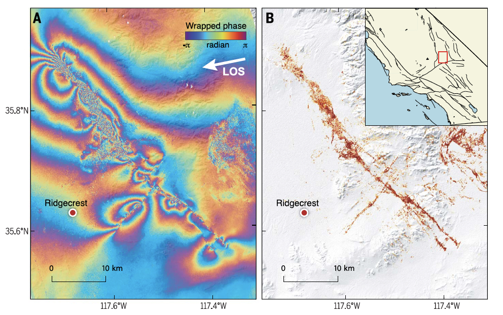
When multiple faults break at different orientations during a single earthquake, seismometers record the complex signatures these events produce. To deduce how such earthquakes propagate through time and space without assuming fault geometry, seismologists can model these earthquakes as several smaller hypothetical quakes called “sub-events.” Summing the seismic signature of the model sub-events results in a complex seismic signature that can be compared with the measured seismogram from the actual event. Ross and colleagues applied this method to disentangle the history of the two major shocks at Ridgecrest.
The best-fit result for the magnitude 6.4 foreshock involves at least 3 discrete strike-slip faults that slipped over the course of 12 seconds. In this model, a 6-kilometer-long northwest trending fault slipped first, followed by a shorter southwest-trending fault. The rupture then jumped south to a 15-kilometer southwest-trending fault that crosses the trace of what would later become the main fault of the mainshock (Figure 3).
For the magnitude 7.1 mainshock, four sub-events lasting a total of 22 seconds best replicate the actual seismic data. In this model, the first sub-event released most of the energy associated with the earthquake, tearing the ground apart as it propagates to the northwest and southeast simultaneously, Ross explains. The latter three sub-events propagated very slowly to the southeast, with the final sub-event almost 25 kilometers southeast of the first, suggesting the rupture tore the surface in a single direction for much of the duration.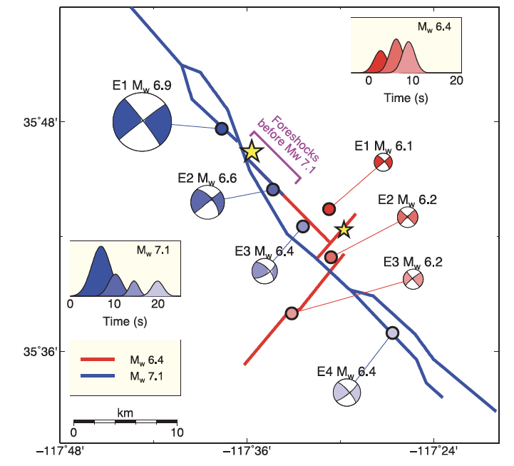
Seismologists worldwide grapple with the question of what limits the size and extent of an earthquake. At Ridgecrest, the magnitude 6.4 event did not trigger immediate slip on the fault that eventually ruptured to produce the magnitude 7.1 mainshock. In fact, no fault area appears to have ruptured twice.
From the hypocenter of the magnitude 6.4 event, the fault trace propagated northwest, stopping 4 kilometers from the eventual magnitude 7.1 hypocenter. This short distance appears to have halted the foreshock’s advance, but in the intervening 34 hours between events, moderately sized shocks chipped away at this seismic barrier. The mainshock may have been triggered simply because an enigmatic line of defense was steadily eroded by smaller foreshocks.
The 260-kilometer-long left-lateral Garlock Fault lies less than 5 kilometers from the southern terminus of the Ridgecrest earthquake sequence. Capable of producing magnitude 7.8 earthquakes, the Garlock fault has been relatively quiet, seismically speaking, with no creep measurable by GPS prior to July of 2019. However, Ross and colleagues found that after the magnitude 6.4 foreshock, a large earthquake swarm was activated along part of the Garlock fault, with greater than 4000 events between magnitude 0 and 3.2 recorded by nearby seismic stations. Further, they found that the Garlock fault also began to creep aseismically as a result of Ridgecrest. If the Garlock fault played a role in limiting the southern extent of faulting, the reason remains a mystery.
The increased resolution afforded by dense seismic networks guides scientists toward a better understanding of earthquake physics while highlighting that the fault database for California is incomplete. The hazards posed by these immature and partly unmapped fault systems, when combined with the challenge of accounting for possible fault combinations that could rupture during an event, underscores the importance of earthquake early warning and preparedness. In short, we may never know where all the faults are, but with appropriate instrumentation and an earthquake early warning system in place, at the very least, we have enough time to drop, cover and hold on.
Figure 1. Map view of seismicity associated with the Ridgecrest earthquake sequence. The colors indicate the earthquake depth. Events with greater than magnitude 4.5 are indicated by beachballs. Black lines show the surface trace of the faults that ruptured during the earthquake sequence, and the purple lines indicate other Quaternary faults. Inset shows map location within Southern California.
The lower panel is a cross section that follows the trace of the main fault of the mainshock, and corresponds to A-A’ in the upper panel. Relocated earthquakes within 1 kilometer of the profile are plotted as a function of depth, with brown lines delineating orthogonal faults. At least 20 individual faults cut this profile. The dashed red line indicates the surface trace of the southwest-trending fault that ruptured in the magnitude 6.4 foreshock, and the solid red line indicates the Garlock Fault. From Ross et al. (2019).
Figure 2 (A). Interferogram derived from comparing before and after satellite images. The before image was collected April 16, 2018, and the after image was collected July 8, 2019, after the magnitude 7.1 mainshock. The color fringes tell scientists which side of a given fault moved up or down relative to the satellite. The line of site (LOS) is the path from the ground to the satellite. (B). Damage proxy map shows where coherence in InSAR data is lost, meaning the color fringes devolve into a seemingly random array of pixels because the ground moved significantly between the pre- and post-seismic images. Darker colors indicate greater coherence loss. From Ross et al. (2019).
Figure 3. In this summary of the best-fit results of the sub-event modeling, the magnitude 6.4 foreshock ruptured 3 main faults. The magnitude 7.1 mainshock had four main sub-events. The magnitudes and beachball diagrams shown near each model sub-event are model results as well. In this analysis, the sum of the magnitudes of the sub-events must equal the total magnitude of the actual event. The foreshocks between the magnitude 6.4 event and the mainshock that appear to have eroded a seismic barrier are noted as well. From Ross et al. (2019).
Cover photo: Scientists examine an area where the Ridgerest earthquake broke the surface. Credit: Katherine Kendrick, USGS. Public domain.
Citation: Ross, Z., et al. (2019) Hierarchical interlocked orthogonal faulting in the 2019 Ridgecrest earthquake sequence, Science, v 366, 346-351. DOI: 10.1126/science.aaz0109