Beneath Alaska’s expanses of ice and wilderness hides a patchwork of terranes stitched together by threads of faults. To explore how the largest U.S. state’s pieces fit together, University of Utah doctoral student Elizabeth Berg used data from earthquakes and the background seismic vibrations of Earth to construct images of the structures below the surface. The techniques she and her colleagues applied, published in the Journal of Geophysical Research:Solid Earth, let them explore the shallow crust, upper mantle, and everything in between. They examined numerous subsurface features ranging from depths of less than a kilometer to more than 100 kilometers down. Berg's models are bringing shallow features into focus, allowing her to image where basin meets bedrock for every major Alaskan basin simultaneously, which is a first for regional-scale studies in this area.
The Earthscope USArray Transportable Array blankets all of Alaska and parts of western Canada with more than 200 seismic stations designed to record Earth's movements at a range of wavelengths, or periods. Waves from earthquakes, including distant ones greater than approximately magnitude-5.0, appear as distinct blips in the lower frequency, higher period part each stations’ seismograms.
The first, fast P-wave, or compressional wave, signals an earthquake. This “body wave” travels through the earth, bouncing off subsurface structures, like the boundary between the crust and mantle, called the Mohorovičić discontinuity. Each bounce produces more P-waves or slower S-waves, also called shear waves, all of which are faithfully recorded by seismic stations. If tomographers can rewind the record of these ricochets, they can calculate the depth of these structures near each station. Berg and her colleagues did just that, deconvolving the waveforms measured at each seismic station for 650 large, distant earthquakes that occurred between January 2015 and August 2018.
Earthquakes also produce surface waves restricted to the upper crust. One type, the Rayleigh wave, moves in multiple planes, rolling through seismic stations with a circular motion. The speed at which Rayleigh waves move through something — called the phase velocity — illuminates different structures, depending on the source. With a bit of calculus, Berg and her colleagues used earthquake-produced Rayleigh waves to “see" 30 to 80 kilometers below each station. To explore shallower depths with similar calculations, Berg used short period data produced by the ceaseless background seismic chatter caused by anything that regularly thumps the earth, like the ocean pounding on the seafloor, called ambient seismic noise. The phase velocity of Rayleigh waves produced by ambient seismic noise showed Berg structures ranging from 10 to 40 kilometers under each station.
In addition to exploiting the speed of Rayleigh waves, Berg used their circularity (or lack thereof), also called ellipticity, calculated from the horizontal and vertical motions recorded at a seismic station. Non-circular, horizontally-elongated, Rayleigh waves must have traveled through a high-contrast boundary, like sediment atop crystalline rock. Rayleigh waves produced by ambient seismic noise probe depths less than one kilometer, making them more sensitive to shallow structures compared to phase velocities for the same period, said Berg, highlighting why using both Rayleigh wave phase velocity and ellipticity produces a more detailed picture of the shallow subsurface.
 Seismic tomographers can determine the structure of the earth by reverse engineering the problem — like a complicated guess and check. They begin with a set of equations meant to model Earth's layers.
In these equations, some values are fixed, but others can vary. By assigning a value to each of these variables, or parameters, from a range of possibilities, tomographers can make predictions to compare with real-world observations, like how P-waves bounce around beneath each station, phase velocity, or ellipticity of Rayleigh waves. Finally, they quantify the comparison by calculating a misfit that signals how far-off from reality the prediction is, ending a single trip through the model.
The most likely model is the one that has the lowest misfit value; it’s the model that can best explain the observations. Berg’s model included 13 parameters that could be changed to decrease misfit.
To find the “best” model from the many hundreds, or even thousands, of possibilities, one option is to randomly select a value from each range of parameters, calculate the prediction and misfit, and repeat the process with a new set of randomly selected parameters many thousands of times. Berg’s method of choice, however, was smarter, letting the previous model’s misfit guide the next model’s parameter selection. Called “Markov Chain Monte Carlo,” this approach requires many fewer trips through possible models before converging on a set of predictions that matches the seismic observations.
Berg first searched for the best combination of model parameters that reproduced all three datasets under each individual seismic station. While this type of analysis reconstructed the column of Earth at each location, the structures between stations remained somewhat mysterious.
To piece together the intervening strata, Berg and her colleagues performed a second analysis, built atop the previous station-by-station one. Here, she says, they “focused on … the phase velocity datasets, as these are sensitive to [the earth’s structures] between stations.” The station-by-station model, extrapolated from the best-fit models fitting all three datasets for 235 stations, Berg says, served as the starting point for this second, entire-region analysis, chopped into 19,407 grid points. For each round through this regional model, Berg explains that she perturbed the parameters ever so slightly to try to further minimize the misfit calculation.
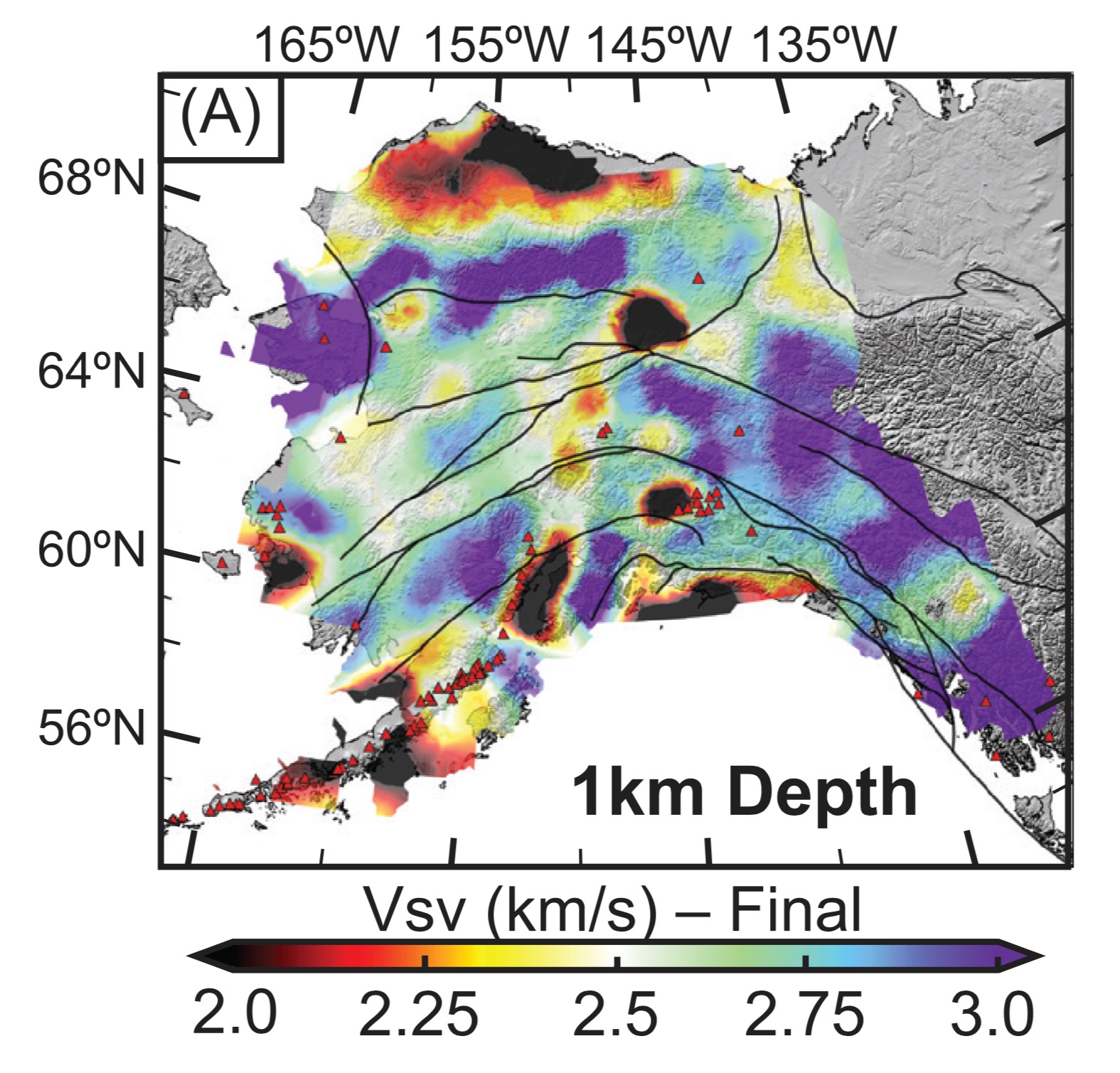
The best-fit result includes a complete map of the shape of at least nine major basins in Alaska, as well as several additional smaller basins throughout the state. These new three-dimensional views will help scientists improve ground motion models in the event of earthquakes, a natural hazard to which many Alaskans are accustomed, because the basin geometry can amplify shaking during large earthquakes. In addition, Berg says, “this work simultaneously takes a snapshot of the basins, volcanic systems, and tectonic plates all interacting miles beneath our feet.”
Figure 1: The final tomographic model at a depth of 1 kilometer, with Holocene and Eocene volcanoes shown as red triangles and major faults drawn as black lines. The color ramp indicates shear wave velocity, with black regions corresponding to near-surface basins throughout Alaska. Credit: Berg et al., 2020.
Cover image: Picture of a Transportable Array Station in Alaska
Citation: Berg, E. M., Lin, F. C., Allam, A., Schulte‐Pelkum, V., Ward, K. M., & Shen, W. (2020). Shear Velocity Model of Alaska Via Joint Inversion of Rayleigh Wave Ellipticity, Phase Velocities, and Receiver Functions Across the Alaska Transportable Array. Journal of Geophysical Research: Solid Earth, 125(2), e2019JB018582.